Francisco Blanco-Silva

Migration

November 11, 2014 Leave a comment

Although I will be keeping this blog for a (long) while up, I will not be adding any other posts or pages in the future.

After much deliberation, I decided to do the migration to a new platform, hosted for free in my github. It involves a great deal of hacking, but in spite of all the extra work, the move is totally worthwhile.

Please, redirect your browser to blancosilva.github.io for my new professional blog.

Categories: Uncategorized

Computational Geometry in Python

September 23, 2014 Leave a comment

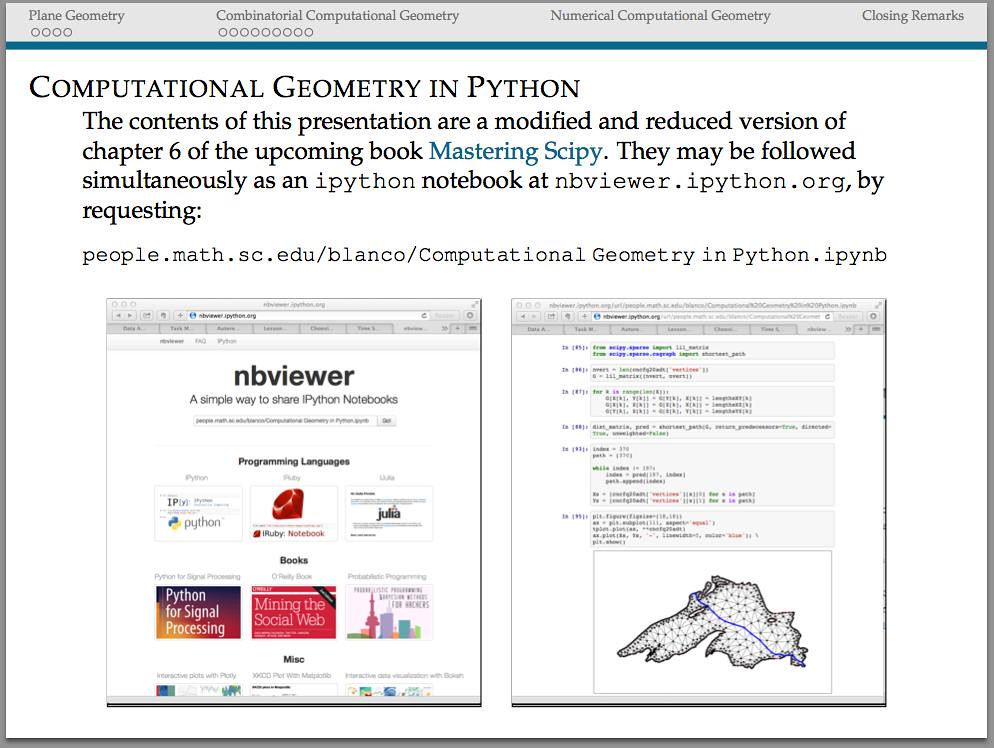
To illustrate a few advantages of the scipy stack in one of my upcoming talks, I have placed an ipython notebook with (a reduced version of) the current draft of Chapter 6 (Computational Geometry) of my upcoming book: Mastering SciPy.

The raw ipynb can be downloaded from my github repository [blancosilva/Mastering-Scipy/], or viewed directly from the nbviewer at [this other link]

I also made a selection with some fun examples for the talk. You can download the presentation by clicking in the image above.

Enjoy!

Searching (again!?) for the SS Central America

August 31, 2014 Leave a comment

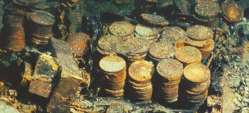
On Tuesday, September 8th 1857, the steamboat SS Central America left Havana at 9 AM for New York, carrying about 600 passengers and crew members. Inside of this vessel, there was stowed a very precious cargo: a set of manuscripts by John James Audubon, and three tons of gold bars and coins. The manuscripts documented an expedition through the yet uncharted southwestern United States and California, and contained 200 sketches and paintings of its wildlife. The gold, fruit of many years of prospecting and mining during the California Gold Rush, was meant to start anew the lives of many of the passengers aboard.

On the 9th, the vessel ran into a storm which developed into a hurricane. The steamboat endured four hard days at sea, and by Saturday morning the ship was doomed. The captain arranged to have women and children taken off to the brig Marine, which offered them assistance at about noon. In spite of the efforts of the remaining crew and passengers to save the ship, the inevitable happened at about 8 PM that same day. The wreck claimed the lives of 425 men, and carried the valuable cargo to the bottom of the sea.

It was not until late 1980s that technology allowed recovery of shipwrecks at deep sea. But no technology would be of any help without an accurate location of the site. In the following paragraphs we would like to illustrate the power of the scipy stack by performing a simple simulation, that ultimately creates a dataset of possible locations for the wreck of the SS Central America, and mines the data to attempt to pinpoint the most probable target.

We simulate several possible paths of the steamboat (say 10,000 randomly generated possibilities), between 7:00 AM on Saturday, and 13 hours later, at 8:00 pm on Sunday. At 7:00 AM on that Saturday the ship’s captain, William Herndon, took a celestial fix and verbally relayed the position to the schooner El Dorado. The fix was 31º25′ North, 77º10′ West. Because the ship was not operative at that point—no engine, no sails—, for the next thirteen hours its course was solely subjected to the effect of ocean current and winds. With enough information, it is possible to model the drift and leeway on different possible paths.

Jotto (5-letter Mastermind) in the NAO robot

July 9, 2014 Leave a comment

I would like to show how to code the NAO robot to beat us at Jotto (5-letter Mastermind) with python in Choregraphe. I will employ a brute force technique that does not require any knowledge of the English language, the frequency of its letters, or smart combinations of vowels and consonants to try to minimize the number of attempts. It goes like this:

Gather all 5-letter words with no repeated letters in a list.
Choose a random word from that list—your guess—, and ask it to be scored ala Mastermind.
Filter through the list all words that share the same score with your guess; discard the rest.
Go back to step 2 and repeat until the target word is found.

Coding this strategy in python requires only four variables:

whole_dict: the list with all the words
step = [x for x in whole_dict]: A copy of whole_dict, which is going to be shortened on each step (hence the name). Note that stating step = whole_dict will change the contents of whole_dict when we change the contents of step — not a good idea.
guess = random.choice(step): A random choice from the list step.
score: A string containing the two digits we obtain after scoring the guess. The first digit indicates the number of correct letters in the same position as the target word; the second digit indicates the number of correct letters in the wrong position.
attempts: optional. The number of attempts at guessing words. For quality control purposes.

At this point, I urge the reader to stop reading the post and try to implement this strategy as a simple script. When done, come back to see how it can be coded in the NAO robot.

Robot stories

June 29, 2014 2 comments

Every summer before school was over, I was assigned a list of books to read. Mostly nonfiction and historical fiction, but in fourth grade there that was that first science fiction book. I often remember how that book made me feel, and marvel at the impact that it had in my life. I had read some science fiction before—Well’s Time Traveller and War of the Worlds—but this was different. This was a book with witty and thought-provoking short stories by Isaac Asimov. Each of them delivered drama, comedy, mystery and a surprise ending in about ten pages. And they had robots. And those robots had personalities, in spite of their very simple programming: The Three Laws of Robotics.

A robot may not injure a human being or, through inaction, allow a human being to come to harm.

A robot must obey the orders given to it by human beings, except where such orders would conflict with the First Law.

A robot must protect its own existence as long as such protection does not conflict with the First or Second Law.

Back in the 1980s, robotics—understood as autonomous mechanical thinking—was no more than a dream. A wonderful dream that fueled many children’s imaginations and probably shaped the career choices of some. I know in my case it did.

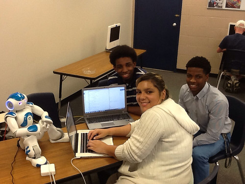
Fast forward some thirty-odd years, when I met Astro: one of three research robots manufactured by the French company Aldebaran. This NAO robot found its way into the computer science classroom of Tom Simpson in Heathwood Hall Episcopal School, and quickly learned to navigate mazes, recognize some student’s faces and names, and even dance the Macarena! It did so with effortless coding: a basic command of the computer language python, and some idea of object oriented programming.

I could not let this opportunity pass. I created a small undergraduate team with Danielle Talley from USC (a brilliant sophomore in computer engineering, with a minor in music), and two math majors from Morris College: my Geometry expert Fabian Maple, and a McGyver-style problem solver, Wesley Alexander. Wesley and Fabian are supported by a Department of Energy-Environmental Management grant to Morris College, which funds their summer research experience at USC. Danielle is funded by the National Science Foundation through the Louis Stokes South Carolina-Alliance for Minority Participation (LS-SCAMP).

They spent the best of their first week on this project completing a basic programming course online. At the same time, the four of us reviewed some of the mathematical tools needed to teach Astro new tricks: basic algebra and trigonometry, basic geometry, and basic calculus and statistics. The emphasis—I need to point out in case you missed it—is in the word basic.

Talk the talk

The psychologist seated herself and watched Herbie narrowly as he took a chair at the other side of the table and went through the three books systematically.

At the end of half an hour, he put them down, “Of course, I know why you brought these.”

The corner of Dr. Calvin’s lip twitched, “I was afraid you would. It’s difficult to work with you, Herbie. You’re always a step ahead of me.”

“It’s the same with these books, you know, as with the others. They just don’t interest me. There’s nothing to your textbooks. Your science is just a mass of collected data plastered together by makeshift theory — and all so incredibly simple, that it’s scarcely worth bothering about.”

“It’s your fiction that interests me. Your studies of the interplay of human motives and emotions” – his mighty hand gestured vaguely as he sought the proper words.

Liar!
— Isaac Asimov

Astro can understand what I say, and maintain conversations with me. He has four microphones for voice recognition and sound localization, and two speakers for text-to-speech synthesis. But he sometimes gets confused: I say “acute”, and he understands “abide,” for example. This might sound frustrating by all standards. But mathematicians can’t be judged by any reasonable standard. Far from seeing this as a shortcoming, my team used as motivation the mechanics behind his speech recognition functionality, and they wrote some code to turn him into an expert Mastermind player.

Wait, what? How are these two things possibly connected?

Since Astro’s hearing is far from perfect, when he hears a word which is not clear, he gathers a short list of possible candidates. He then chooses the most likely guess based upon different considerations—using clues from context, for example. Based on similar strategies, he can be taught to be a perfect player of 5-letter-word Mastermind: Pick any five-letter word in the English language. Any word, provided it has no repeated letters. Astro chooses one random word as his first guess, and requests a score like in Mastermind.

To illustrate this process, I will show you how the game went when I chose Fabian’s favorite word: “acute.”

Astro: Is it firth?
Me   : NO
Astro: How many letters of my guess are in your word, in the right position?
       How many letters of my guess are in your word, in the wrong position?
Me   : 1, 0
Astro: Is it foams?
Me   : NO
Astro: How many letters of my guess are in your word, in the right position?
       How many letters of my guess are in your word, in the wrong position?
Me   : 0, 1
Astro: Is it junta?
Me   : NO
Astro: How many letters of my guess are in your word, in the right position?
       How many letters of my guess are in your word, in the wrong position?
Me   : 1, 2
Astro: Is it acute?
Me   : YES
Astro: Wonderful, I found it in 4 attempts!

I don’t want to get too technical here, but will mention some of the ideas. The main algorithm is based on techniques of numerical root finding and solving nonlinear equations — nothing complex: high-school level bracketing by bisection, or Newton’s method. To design better winning strategies, my team exploits the benefits of randomness. The analysis of this part is done with basic probability and statistics.

Walk the walk

Donovan’s pencil pointed nervously. “The red cross is the selenium pool. You marked it yourself.”

“Which one is it?” interrupted Powell. “There were three that MacDougal located for us before he left.”

“I sent Speedy to the nearest, naturally; seventeen miles away. But what difference does that make?” There was tension in his voice. “There are penciled dots that mark Speedy’s position.”

And for the first time Powell’s artificial aplomb was shaken and his hands shot forward for the man.

“Are you serious? This is impossible.”

“There it is,” growled Donovan.

The little dots that marked the position formed a rough circle about the red cross of the selenium pool. And Powell’s fingers went to his brown mustache, the unfailing signal of anxiety.

Donovan added: “In the two hours I checked on him, he circled that damned pool four times. It seems likely to me that he’ll keep that up forever. Do you realize the position we’re in?”

Runaround
— Isaac Asimov

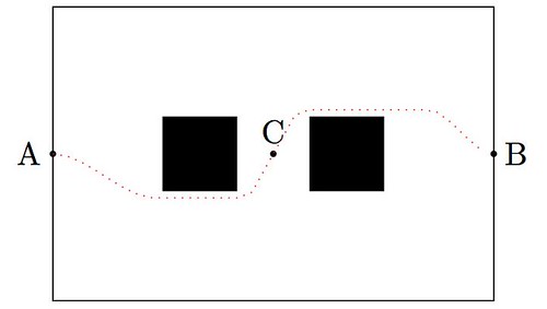
Astro moves around too. It does so thanks to a sophisticated system combining one accelerometer, one gyrometer and four ultrasonic sensors that provide him with stability and positioning within space. He also enjoys eight force-sensing resistors and two bumpers. And that is only for his legs! He can move his arms, bend his elbows, open and close his hands, or move his torso and neck (up to 25 degrees of freedom for the combination of all possible joints). Out of the box, and without much effort, he can be coded to walk around, although in a mechanical way: He moves forward a few feet, stops, rotates in place or steps to a side, etc. A very naïve way to go from A to B retrieving an object at C, could be easily coded in this fashion as the diagram shows:

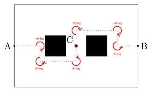
Fabian and Wesley devised a different way to code Astro taking full advantage of his inertial measurement unit. This will allow him to move around smoothly, almost like a human would. The key to their success? Polynomial interpolation and plane geometry. For advanced solutions, they need to learn about splines, curvature, and optimization. Nothing they can’t handle.

Sing me a song

He said he could manage three hours and Mortenson said that would be perfect when I gave him the news. We picked a night when she was going to be singing Bach or Handel or one of those old piano-bangers, and was going to have a long and impressive solo.

Mortenson went to the church that night and, of course, I went too. I felt responsible for what was going to happen and I thought I had better oversee the situation.

Mortenson said, gloomily, “I attended the rehearsals. She was just singing the same way she always did; you know, as though she had a tail and someone was stepping on it.”

One Night of Song
— Isaac Asimov

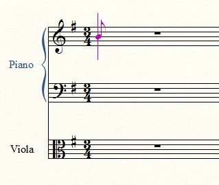
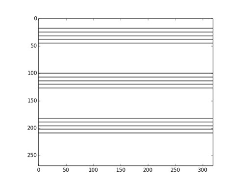
Astro has excellent eyesight and understanding of the world around him. He is equipped with two HD cameras, and a bunch of computer vision algorithms, including facial and shape recognition. Danielle’s dream is to have him read from a music sheet and sing or play the song in a toy piano. She is very close to completing this project: Astro is able now to identify partitures, and extract from them the location of the pentagrams. Danielle is currently working on identifying the notes and the clefs. This is one of her test images, and the result of one of her early experiments:

https://farm3.staticflickr.com/2906/14350961337_97bcb90e88_o_d.jpg

https://farm4.staticflickr.com/3856/14537520835_4f0bf31eb1_d.jpg

Most of the techniques Danielle is using are accessible to any student with a decent command of vector calculus, and enough scientific maturity. The extraction of pentagrams and the different notes on them, for example, is performed with the Hough transform. This is a fancy term for an algorithm that basically searches for straight lines and circles by solving an optimization problem in two or three variables.

The only thing left is an actual performance. Danielle will be leading Fabian and Wes, and with the assistance of Mr. Simpson’s awesome students Erica and Robert, Astro will hopefully learn to physically approach the piano, choose the right keys, and play them in the correct order and speed. Talent show, anyone?

Advanced Problem #18

March 4, 2014 Leave a comment

Another fun problem, as requested by Qinfeng Li in MA598R: Measure Theory

Let $f \in L_2(\mathbb{R})$ so that $g(x)=xf(x) \in L_2(\mathbb{R})$ too.

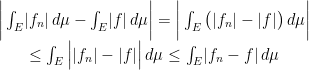
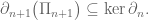
Show that $f \in L_1(\mathbb{R})$ and $\lVert f \rVert_1^2 \leq 8 \lVert f \rVert_2 \lVert g \rVert_2.$

I got this problem by picking some strictly positive value $\lambda$ and breaking the integral $\int_{\mathbb{R}} \lvert f \rvert\, d\mu$ as follows:

$\begin{array}{rl} \displaystyle{\int_{\mathbb{R}} \lvert f \rvert\, d\mu} &= \displaystyle{\int_{\lvert x \rvert \leq \lambda} \lvert f \rvert\, d\mu + \int_{\lvert x \rvert \geq \lambda} \lvert f \rvert\, d\mu} \\ \\ &= \displaystyle{\int_{-\lambda}^{\lambda} \lvert f \rvert\, d\mu + \int_{\lvert x \rvert \geq \lambda} \tfrac{1}{\lvert x \rvert} \lvert g(x) \rvert\, d\mu} \\ \\ &= \displaystyle{\int_\mathbb{R} \lvert f \rvert \cdot \boldsymbol{1}_{\lvert x \rvert \leq \lambda}\, d\mu + \int_{\mathbb{R}} \lvert g \rvert \cdot \big( \tfrac{1}{\lvert x \rvert} \boldsymbol{1}_{\lvert x \rvert \geq \lambda}\big) \, d\mu} \\ \\ &\leq \lVert f \rVert_2 \cdot \big\lVert \boldsymbol{1}_{\lvert x \rvert \leq \lambda} \big\rVert_2 + \lVert g \rVert_2 \cdot \big\lVert \tfrac{1}{\lvert x \rvert} \boldsymbol{1}_{\lvert x \rvert \geq \lambda} \big\rVert_2 \end{array}$

Let us examine now the factors $\big\lVert \boldsymbol{1}_{\lvert x \rvert \leq \lambda} \big\rVert_2$ and $\big\lVert \tfrac{1}{\lvert x \rvert} \boldsymbol{1}_{\lvert x \rvert \geq \lambda} \big\rVert_2$ above:

$\big\lVert \boldsymbol{1}_{\lvert x \rvert \leq \lambda} \big\rVert_2 = \sqrt{2\lambda}$

$\big\lVert \tfrac{1}{\lvert x \rvert} \boldsymbol{1}_{\lvert x \rvert \geq \lambda} \big\rVert_2 = \displaystyle{ \sqrt{ 2\int_\lambda^\infty \dfrac{dx}{x^2}} = \sqrt{ \dfrac{2}{\lambda}} }$

We have thus proven that $f \in L_1(\mathbb{R})$ with $\lVert f \rVert_1 \leq \sqrt{2\lambda} \lVert f \rVert_2 + \sqrt{\tfrac{2}{\lambda}} \lVert g \rVert_2.$ At this point, all you have to do is pick $\lambda = \lVert g \rVert_2 / \lVert f \rVert_2$ (provided the denominator is not zero) and you are done.

Categories: Analysis, puzzles, Teaching

Book presentation at the USC Python Users Group

December 7, 2013 Leave a comment

Areas of Mathematics

October 22, 2013 3 comments

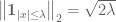
For one of my upcoming talks I am trying to include an exhaustive mindmap showing the different areas of Mathematics, and somehow, how they relate to each other. Most of the information I am using has been processed from years of exposure in the field, and a bit of help from Wikipedia.

But I am not entirely happy with what I see: my lack of training in the area of Combinatorics results in a rather dry treatment of that part of the mindmap, for example. I am afraid that the same could be told about other parts of the diagram. Any help from the reader to clarify and polish this information will be very much appreciated.

And as a bonus, I included a $\LaTeX$ script to generate the diagram with the aid of the tikz libraries.

\tikzstyle{level 2 concept}+=[sibling angle=40]
\begin{tikzpicture}[scale=0.49, transform shape]
  \path[mindmap,concept color=black,text=white]
    node[concept] {Pure Mathematics} [clockwise from=45]
      child[concept color=DeepSkyBlue4]{
        node[concept] {Analysis} [clockwise from=180]
          child { 
            node[concept] {Multivariate \& Vector Calculus}
              [clockwise from=120]
              child {node[concept] {ODEs}}}
              child { node[concept] {Functional Analysis}}
              child { node[concept] {Measure Theory}}
              child { node[concept] {Calculus of Variations}}
              child { node[concept] {Harmonic Analysis}}
              child { node[concept] {Complex Analysis}}
              child { node[concept] {Stochastic Analysis}}
              child { node[concept] {Geometric Analysis}
                [clockwise from=-40]
                child {node[concept] {PDEs}}}}
          child[concept color=black!50!green, grow=-40]{ 
            node[concept] {Combinatorics} [clockwise from=10]
              child {node[concept] {Enumerative}}
              child {node[concept] {Extremal}}
              child {node[concept] {Graph Theory}}}
          child[concept color=black!25!red, grow=-90]{ 
            node[concept] {Geometry} [clockwise from=-30]
              child {node[concept] {Convex Geometry}}
              child {node[concept] {Differential Geometry}}
              child {node[concept] {Manifolds}}
              child {node[concept,color=black!50!green!50!red,text=white] {Discrete Geometry}}
              child {
                node[concept] {Topology} [clockwise from=-150]
                  child {node [concept,color=black!25!red!50!brown,text=white]
                    {Algebraic Topology}}}}
          child[concept color=brown,grow=140]{ 
            node[concept] {Algebra} [counterclockwise from=70]
              child {node[concept] {Elementary}}
              child {node[concept] {Number Theory}}
              child {node[concept] {Abstract} [clockwise from=180]
                child {node[concept,color=red!25!brown,text=white] {Algebraic Geometry}}}
              child {node[concept] {Linear}}}
    node[extra concept,concept color=black] at (200:5) {Applied Mathematics} 
      child[grow=145,concept color=black!50!yellow] {
        node[concept] {Probability} [clockwise from=180]
          child {node[concept] {Stochastic Processes}}}
      child[grow=175,concept color=black!50!yellow] {node[concept] {Statistics}}
      child[grow=205,concept color=black!50!yellow] {node[concept] {Numerical Analysis}}
      child[grow=235,concept color=black!50!yellow] {node[concept] {Symbolic Computation}};
\end{tikzpicture}

More on Lindenmayer Systems

September 24, 2013 2 comments

We briefly explored Lindenmayer systems (or L-systems) in an old post: Toying with Basic Fractals. We quickly reviewed this method for creation of an approximation to fractals, and displayed an example (the Koch snowflake) based on tikz libraries.

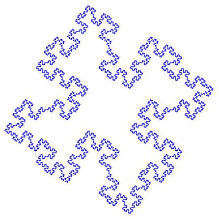
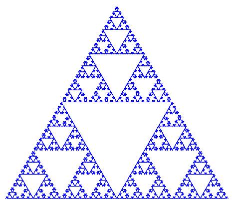
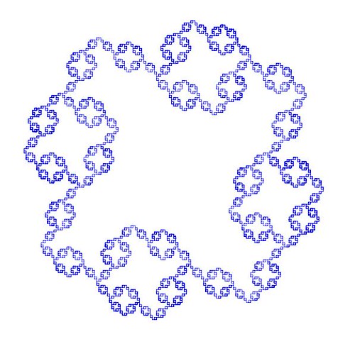
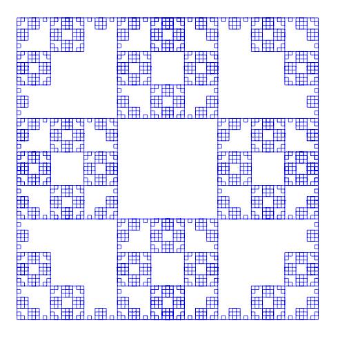
I would like to show a few more examples of beautiful curves generated with this technique, together with their generating axiom, rules and parameters. Feel free to click on each of the images below to download a larger version.

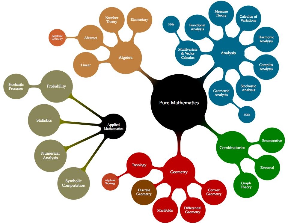
Note that any coding language with plotting capabilities should be able to tackle this project. I used once again tikz for $\text{\LaTeX}$ , but this time with the tikzlibrary lindenmayersystems.


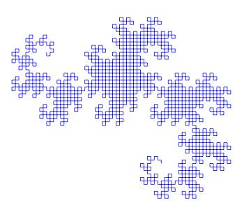
name : Dragon Curve axiom : X order : 11 step : 5pt angle : 90 rules : X -> X+YF+ Y -> -FX-Y	name : Gosper Space-filling Curve axiom : XF order : 5 step : 2pt angle : 60 rules : XF -> XF+YF++YF-XF--XFXF-YF+ YF -> -XF+YFYF++YF+XF--XF-YF

name : Quadric Koch Island axiom : F+F+F+F order : 4 step : 1pt angle : 90 rules : F -> F+F-F-FF+F+F-F	name : Sierpinski Arrowhead axiom : F order : 8 step : 3.5pt angle : 60 rules : G -> F+G+F F -> G-F-G

name : ? axiom : F+F+F+F order : 4 step : 2pt angle : 90 rules : F -> FF+F+F+F+F+F-F	name : ? axiom : F+F+F+F order : 4 step : 3pt angle : 90 rules : F -> FF+F+F+F+FF

Would you like to experiment a little with axioms, rules and parameters, and obtain some new pleasant curves with this method? If the mathematical properties of the fractal that they approximate are interesting enough, I bet you could attach your name to them. Like the astronomer that finds through her telescope a new object in the sky, or the zoologist that discover a new species of spider in the forest.

Categories: Geometry, Imaging, Linear Algebra, puzzles, Python, Scientific Computing, TeX/LaTeX Tags: fractal, Gosper, Koch, L-system, LaTeX, Lindenmayer system, python, Sierpinski, Space-filling curves, tikz

Some results related to the Feuerbach Point

July 15, 2013 Leave a comment

Given a triangle $\triangle ABC,$ the circle that goes through the midpoints of each side, $D, E, F,$ is called the Feuerbach circle. It has very surprising properties:

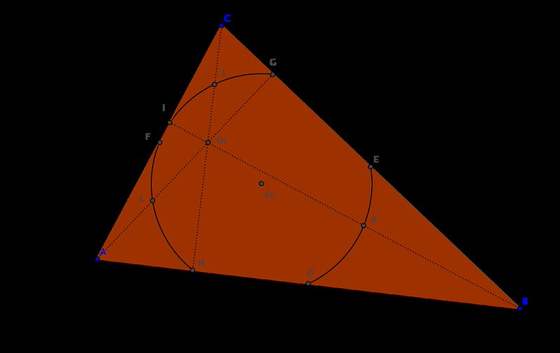
It also goes through the feet of the heights, points $G, H, I.$
If $Oc$ denotes the orthocenter of the triangle, then the Feuerbach circle also goes through the midpoints of the segments $OcA, OcB, OcC.$ For this reason, the Feuerbach circle is also called the nine-point circle.
The center of the Feuerbach circle is the midpoint between the orthocenter and circumcenter of the triangle.
The area of the circumcircle is precisely four times the area of the Feuerbach circle.

Most of these results are easily shown with sympy without the need to resort to Gröbner bases or Ritt-Wu techniques. As usual, we realize that the properties are independent of rotation, translation or dilation, and so we may assume that the vertices of the triangle are $A=(0,0), B=(1,0)$ and $C=(r,s)$ for some positive parameters $r,s>0.$ To prove the last statement, for instance we may issue the following:

>>> import sympy
>>> from sympy import *
>>> A=Point(0,0)
>>> B=Point(1,0)
>>> r,s=var('r,s')
>>> C=Point(r,s)
>>> D=Segment(A,B).midpoint
>>> E=Segment(B,C).midpoint
>>> F=Segment(A,C).midpoint
>>> simplify(Triangle(A,B,C).circumcircle.area/Triangle(D,E,F).circumcircle.area)
4

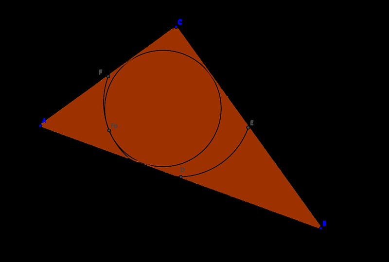
But probably the most amazing property of the nine-point circle, is the fact that it is tangent to the incircle of the triangle. With exception of the case of equilateral triangles, both circles intersect only at one point: the so-called Feuerbach point.

An Automatic Geometric Proof

July 9, 2013 4 comments

We are familiar with that result that states that, on any given triangle, the circumcenter, centroid and orthocenter are always collinear. I would like to illustrate how to use Gröbner bases theory to prove that the incenter also belongs in the previous line, provided the triangle is isosceles.

We start, as usual, indicating that this property is independent of shifts, rotations or dilations, and therefore we may assume that the isosceles triangle has one vertex at $A=(0,0)$ , another vertex at $B=(1,0)$ and the third vertex at $C=(1/2, s)$ for some value $s \neq 0.$ In that case, we will need to work on the polynomial ring $R=\mathbb{R}[s,x_1,x_2,x_3,y_1,y_2,y_3,z],$ since we need the parameter $s$ free, the variables $x_1$ and $y_1$ are used to input the conditions for the circumcenter of the triangle, the variables $x_2$ and $y_2$ for centroid, and the variables $x_3$ and $y_3$ for the incenter (note that we do not need to use the orthocenter in this case).

We may obtain all six conditions by using sympy, as follows:

>>> import sympy
>>> from sympy import *
>>> A=Point(0,0)
>>> B=Point(1,0)
>>> s=symbols("s",real=True,positive=True)
>>> C=Point(1/2.,s)
>>> T=Triangle(A,B,C)
>>> T.circumcenter
Point(1/2, (4*s**2 - 1)/(8*s))
>>> T.centroid
Point(1/2, s/3)
>>> T.incenter
Point(1/2, s/(sqrt(4*s**2 + 1) + 1))

This translates into the following polynomials

$h_1=2x_1-1, h_2=8sy_1-4s^2+1$ (for circumcenter)
$h_3=2x_2-1, h_4=3y_2-s$ (for centroid)
$h_5=2x_3-1, h_6=(4sy_3+1)^2-4s^2-1$ (for incenter)

The hypothesis polynomial comes simply from asking whether the slope of the line through two of those centers is the same as the slope of the line through another choice of two centers; we could use then, for example, $g=(x_2-x_1)(y_3-y_1)-(x_3-x_1)(y_2-y_1).$ It only remains to compute the Gröbner basis of the ideal $I=(h_1, \dotsc, h_6, 1-zg) \subset \mathbb{R}[s,x_1,x_2,x_3,y_1,y_2,y_3,z].$ Let us use SageMath for this task:

sage: R.<s,x1,x2,x3,y1,y2,y3,z>=PolynomialRing(QQ,8,order='lex')
sage: h=[2*x1-1,8*r*y1-4*r**2+1,2*x2-1,3*y2-r,2*x3-1,(4*r*y3+1)**2-4*r**2-1]
sage: g=(x2-x1)*(y3-y1)-(x3-x1)*(y2-y1)
sage: I=R.ideal(1-z*g,*h)
sage: I.groebner_basis()
[1]

This proves the result.

Categories: Algebra, Geometry, Linear Algebra, Python, sage, Scientific Computing, Teaching Tags: centroid, circumcenter, geometry, Groebner, Groebner basis, incenter, orthocenter, triangle

Sympy should suffice

June 6, 2013 Leave a comment

I have just received a copy of Instant SymPy Starter, by Ronan Lamy—a no-nonsense guide to the main properties of SymPy, the Python library for symbolic mathematics. This short monograph packs everything you should need, with neat examples included, in about 50 pages. Well-worth its money.

To celebrate, I would like to pose a few coding challenges on the use of this library, based on a fun geometric puzzle from cut-the-knot: Rhombus in Circles

Segments $\overline{AB}$ and $\overline{CD}$ are equal. Lines $AB$ and $CD$ intersect at $M.$ Form four circumcircles: $(E)=(ACM), (F)=(ADM), (G)=(BDM), (H)=(BCM).$ Prove that the circumcenters $E, F, G, H$ form a rhombus, with $\angle EFG = \angle AMC.$

Note that if this construction works, it must do so independently of translations, rotations and dilations. We may then assume that $M$ is the origin, that the segments have length one, $A=(2,0), B=(1,0),$ and that for some parameters $a>0, \theta \in (0, \pi),$ it is $C=(a+1) (\cos \theta, \sin\theta), D=a (\cos\theta, \sin\theta).$ We let SymPy take care of the computation of circumcenters:

import sympy
from sympy import *

# Point definitions
M=Point(0,0)
A=Point(2,0)
B=Point(1,0)
a,theta=symbols('a,theta',real=True,positive=True)
C=Point((a+1)*cos(theta),(a+1)*sin(theta))
D=Point(a*cos(theta),a*sin(theta))

#Circumcenters
E=Triangle(A,C,M).circumcenter
F=Triangle(A,D,M).circumcenter
G=Triangle(B,D,M).circumcenter
H=Triangle(B,C,M).circumcenter

Finding that the alternate angles are equal in the quadrilateral $EFGH$ is pretty straightforward:

In [11]: P=Polygon(E,F,G,H)

In [12]: P.angles[E]==P.angles[G]
Out[12]: True

In [13]: P.angles[F]==P.angles[H]
Out[13]: True

To prove it a rhombus, the two sides that coincide on each angle must be equal. This presents us with the first challenge: Note for example that if we naively ask SymPy whether the triangle $\triangle EFG$ is equilateral, we get a False statement:

In [14]: Triangle(E,F,G).is_equilateral()
Out[14]: False

In [15]: F.distance(E)
Out[15]: Abs((a/2 - cos(theta))/sin(theta) - (a - 2*cos(theta) + 1)/(2*sin(theta)))

In [16]: F.distance(G)
Out[16]: sqrt(((a/2 - cos(theta))/sin(theta) - (a - cos(theta))/(2*sin(theta)))**2 + 1/4)

Part of the reason is that we have not indicated anywhere that the parameter theta is to be strictly bounded above by $\pi$ (we did indicate that it must be strictly positive). The other reason is that SymPy does not handle identities well, unless the expressions to be evaluated are perfectly simplified. For example, if we trust the routines of simplification of trigonometric expressions alone, we will not be able to resolve this problem with this technique:

In [17]: trigsimp(F.distance(E)-F.distance(G),deep=True)==0
Out[17]: False

Finding that $\angle EFG = \angle AMC$ with SymPy is not that easy either. This is the second challenge.

How would the reader resolve this situation?

Instant SymPy Starter

Categories: Geometry, puzzles, sage, Teaching Tags: circumcenter, cuttheknot, geometry, puzzles, python, rhombus, sympy, triangle

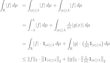
A nice application of Fatou’s Lemma

June 1, 2013 Leave a comment

Let me show you an exciting technique to prove some convergence statements using exclusively functional inequalities and Fatou’s Lemma. The following are two classic problems solved this way. Enjoy!

Exercise 1 Let ${(X, \mathcal{F}, \mu)}$ be a measurable space and suppose ${\{f_n\}_{n\in \mathbb{N}}}$ is a sequence of measurable functions in ${L_1(\mu)}$ that converge almost everywhere to a function ${f \in L_1(\mu)},$ and such that the sequence of norms ${\big\{ \lVert f_n \rVert_1 \big\}_{n \in \mathbb{N}}}$ converges to ${\lVert f \rVert_1}$ . Prove that the sequence of integrals ${\int_E \lvert f_n \rvert\, d\mu}$ converges to the integral ${\int_E \lvert f \rvert\, d\mu}$ for every measurable set ${E}$ .

Proof: Note first that

$\displaystyle \begin{array}{rcl} \lvert f_n - f\rvert\, \boldsymbol{1}_E \leq \lvert f_n - f \rvert \leq \lvert f_n \rvert + \lvert f \rvert. \end{array}$

Set then ${g_n = \lvert f_n \rvert + \lvert f \rvert - \lvert f_n-f \rvert\, \boldsymbol{1}_E}$ (which are non-negative functions) and apply Fatou’s Lemma to that sequence. We have then

$\displaystyle \begin{array}{c} \int_X \liminf_n g_n\, d\mu \leq \liminf_n \int_X g_n\, d\mu \\ \\ \int_X \liminf_n \big( \lvert f_n \rvert + \lvert f \rvert - \lvert f_n - f \rvert\, \boldsymbol{1}_E \big)\, d\mu \leq \liminf_n \int_X \big( \lvert f_n \rvert + \lvert f \rvert - \lvert f_n - f \rvert\, \boldsymbol{1}_E \big)\, d\mu \\ \\ \int_X \big( 2\lvert f \rvert - \limsup_n \lvert f_n-f \rvert\, \boldsymbol{1}_E\big)\, d\mu \leq \liminf_n \int_X \lvert f_n \rvert\, d\mu + \lVert f \rVert_1 - \limsup_n \int_E \lvert f_n -f \rvert\, d\mu \\ \\ 2\lVert f\rVert_1 \leq 2\lVert f \rVert_1 - \limsup_n \int_E \lvert f_n - f\rvert\, d\mu, \end{array}$

which implies

$\displaystyle \begin{array}{rcl} 0 \leq \liminf_n \int_E \lvert f_n-f \rvert\, d\mu \leq \limsup_n \int_E \lvert f_n-f \rvert\, d\mu \leq 0. \end{array}$

It must then be ${\int_E \lvert f_n - f \rvert\, d\mu = 0}$ . But this proves the statement, since

$\displaystyle \begin{array}{c} \bigg\lvert \int_E \lvert f_n\rvert\, d\mu - \int_E \lvert f \rvert\, d\mu \bigg\rvert = \bigg\lvert \int_E \big( \lvert f_n \rvert - \lvert f \rvert \big)\, d\mu \bigg\rvert \\ \leq \int_E \Big\lvert \lvert f_n \rvert - \lvert f \rvert \Big\rvert\, d\mu \leq \int_E \lvert f_n - f \rvert\, d\mu \end{array}$

$\Box$

Exercise 2 Let ${(X, \mathcal{F}, \mu)}$ be a finite measure space and let ${1<p<\infty}$ . Suppose that ${\{ f_n \}_{n \in \mathbb{N}}}$ is a sequence of measurable functions in ${L_p(\mu)}$ whose norms are uniformly bounded in ${n}$ and which converge almost everywhere to a function ${f}$ . Prove that the sequence ${\big\{ \int_X f_ng\, d\mu \big\}_{n \in \mathbb{N}}}$ converges to ${\int_x fg\, d\mu}$ for all ${g \in L_q(\mu)}$ where ${q}$ is the conjugate exponent of ${p}$ .

Proof: The proof is very similar to the previous problem. We start by noticing that under the hypotheses of the problem,

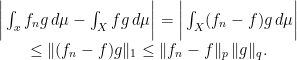
$\displaystyle \begin{array}{c} \bigg\lvert \int_x f_ng\, d\mu - \int_X fg\, d\mu \bigg\rvert = \bigg\lvert \int_X (f_n -f)g\, d\mu \bigg\rvert \\ \leq \lVert (f_n-f)g \rVert_1 \leq \lVert f_n - f \rVert_p\, \lVert g \rVert_q. \end{array}$

If we prove that ${\lim_n \lVert f_n-f \rVert_p = 0}$ , we are done.

We will achieve this by using the convexity of ${\lvert \cdot \rvert^p}$ , since in that case it is

$\displaystyle \begin{array}{rcl} \frac{\lvert f_n - f \rvert^p}{2^p} \leq \tfrac{1}{2} \lvert f_n \rvert^p + \tfrac{1}{2} \lvert f \rvert^p. \end{array}$

hence,

$\displaystyle \begin{array}{rcl} \lvert f_n -f \rvert^p \leq 2^{p-1} \big( \lvert f_n \rvert^p + \lvert f \rvert^p \big). \end{array}$

Set then ${g_n = 2^{p-1} \big( \lvert f_n\rvert^p + \lvert f \rvert^p\big) - \lvert f_n-f \rvert^p}$ (which are non-negative functions) and apply Fatou’s Lemma as before. $\Box$

Categories: Analysis, Teaching Tags: Fatou's Lemma, Measure Theory, Real Analysis

Have a child, plant a tree, write a book

April 23, 2013 2 comments

Or more importantly: rear your children to become nice people, water those trees, and make sure that your books make a good impact.

I recently enjoyed the rare pleasure of having a child (my first!) and publishing a book almost at the same time. Since this post belongs in my professional blog, I will exclusively comment on the latter: Learning SciPy for Numerical and Scientific Computing, published by Packt in a series of technical books focusing on Open Source software.

Keep in mind that the book is for a very specialized audience: not only do you need a basic knowledge of Python, but also a somewhat advanced command of mathematics/physics, and an interest in engineering or scientific applications. This is an excerpt of the detailed description of the monograph, as it reads in the publisher’s page:

It is essential to incorporate workflow data and code from various sources in order to create fast and effective algorithms to solve complex problems in science and engineering. Data is coming at us faster, dirtier, and at an ever increasing rate. There is no need to employ difficult-to-maintain code, or expensive mathematical engines to solve your numerical computations anymore. SciPy guarantees fast, accurate, and easy-to-code solutions to your numerical and scientific computing applications.

Learning SciPy for Numerical and Scientific Computing unveils secrets to some of the most critical mathematical and scientific computing problems and will play an instrumental role in supporting your research. The book will teach you how to quickly and efficiently use different modules and routines from the SciPy library to cover the vast scope of numerical mathematics with its simplistic practical approach that is easy to follow.

The book starts with a brief description of the SciPy libraries, showing practical demonstrations for acquiring and installing them on your system. This is followed by the second chapter which is a fun and fast-paced primer to array creation, manipulation, and problem-solving based on these techniques.

The rest of the chapters describe the use of all different modules and routines from the SciPy libraries, through the scope of different branches of numerical mathematics. Each big field is represented: numerical analysis, linear algebra, statistics, signal processing, and computational geometry. And for each of these fields all possibilities are illustrated with clear syntax, and plenty of examples. The book then presents combinations of all these techniques to the solution of research problems in real-life scenarios for different sciences or engineering — from image compression, biological classification of species, control theory, design of wings, to structural analysis of oxides.

The book is also being sold online in Amazon, where it has been received with pretty good reviews. I have found other random reviews elsewhere, with similar welcoming comments:

Artificial Intelligence in Motion by Marcel Caraciolo
The Endeavour, by John D. Cook

Categories: Analysis, Approximation Theory, Books, Combinatorics, Data mining, differential equations, Geometry, Imaging, Linear Algebra, Probability, Scientific Computing, Statistics

Project Euler with Julia

January 4, 2013 Leave a comment

Disclaimer: Project Euler discourages the posting of solutions to their problems, to avoid spoilers. The three solutions I have presented in my blog are to the three first problems (the easiest and most popular), as a means to advertise and encourage my readers to “push the envelope” and go beyond brute-force solutions.

Just for fun, and as a means to learn Julia, I will be attempting problems from the Project Euler coding exclusively in that promising computer language.

The first problem is very simple:

Multiples of 3 and 5
If we list all the natural numbers below 10 that are multiples of 3 or 5, we get 3, 5, 6 and 9. The sum of these multip les is 23.

Find the sum of all the multiples of 3 or 5 below 1000.

One easy-to-code way is by dealing with arrays:

julia> sum( filter( x->((x%3==0) | (x%5==0)), [1:999] ) )
233168

A much better way is to obtain it via summation formulas: Note that the sum of all multiples of three between one and 999 is given by

$3+6+\dotsb+999 = 3 (1+2+\dotsb+333) = 3 \frac{333\cdot 334}{2} = 166833.$

Similarly, the sum of all multiples of five between one and 995 is given by

$5+10+\dotsb+995 = 5 (1+2+\dotsb+199) = 5 \frac{199\cdot 200}{2} = 99500.$

Finally, we need to subtract the sum of the multiples of both three and five, since they have been counted twice. This sum is

$15+30+\dotsb+990 = 15 (1+2+\dotsb+66)= 15 \frac{66\cdot 67}{2}= 33165.$

The final sum is then, $166833+99500-33165=233168.$

Categories: puzzles Tags: coding, Julia, programming, project Euler, puzzles

Seked

December 16, 2012 Leave a comment

If a pyramid is 250 cubits high and the side of its base 360 cubits long, what is its seked?

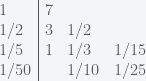
Take half of 360; it makes 180. Multiply 250 so as to get 180; it makes $1/2 1/5 1/50$ of a cubit. A cubit is 7 palms. Multiply 7 by $1/2 1/5 1/50:$

$\begin{array}{l|lll} 1&7&&\\ 1/2&3&1/2& \\ 1/5 &1&1/3&1/15\\ 1/50&&1/10&1/25 \end{array}$

The seked is $5 \tfrac{1}{25}$ palms [that is, $(3+1/2) + (1+1/3+1/15) + (1/10+1/25)$ ].

A’h-mose. The Rhind Papyrus. 33 AD

The image above presents one of the problems included in the Rhind Papyrus, written by the scribe Ahmes (A’h-mose) circa 33 AD. This is a description of all the hieroglyphs, as translated by August Eisenlohr:

The question for the reader, after going carefully over the English translation is: What does seked mean?

Categories: History, puzzles Tags: Egypt, hieroglyphs, history of math, papyrus, puzzles, trigonometry

Nezumi San

December 14, 2012 Leave a comment

On January first, a pair of mice appeared in a house and bore six male mice and six female mice. At the end of January there are fourteen mice: seven male and seven female.

On the first of February, each of the seven pairs bore six male and six female mice, so that at the end of February there are ninety-eight mice in forty-nine pairs. From then on, each pair of mice bore six more pairs every month.

Find the number of mice at the end of December.

Assume that the length of each mouse is 4 sun. If all the mice line up, each biting the tail of the one in front, find the total length of mice

Jinkō-ki, 1715

Categories: History, puzzles Tags: history of math, Japan, puzzles

Ruthless Thieves Stealing a Roll of Cloth

December 14, 2012 Leave a comment

Some thieves stole a long roll of silk cloth from a warehouse. In a bush far from the warehouse, they counted the length of the cloth. If each thief gets 6 hiki, then 6 hiki is left over, but if each thief takes 7 hiki then the last thief gets no cloth at all. Find the number of thieves and the length of the cloth.

Jinkō-ki, 1643

Categories: History, puzzles Tags: history of math, Japan, puzzles

Which one is the fake?

December 7, 2012 5 comments


“Crab on its back”	“Willows at sunset”	“Still life: Potatoes in a yellow dish”

Categories: Approximation Theory, Data mining, Imaging, Probability, puzzles, Scientific Computing, Statistics Tags: approximation theory, art authentication, curvelets, data mining, Daubechies, scientific computing, shearlets, statistics, Van Gogh, wavelets

Stones, balances, matrices

August 7, 2012 Leave a comment

Let’s examine an easy puzzle on finding the different stone by using a balance:

You have four stones identical in size and appearance, but one of them is heavier than the rest. You have a set of scales (a balance): how many weights do you need to determine which stone is the heaviest?

This is a trivial problem, but I will use it to illustrate different ideas, definitions, and the connection to linear algebra needed to answer the harder puzzles below. Let us start by solving it in the most natural way:

Enumerate each stone from 1 to 4.
Set stones 1 and 2 on the left plate; set stones 3 and 4 on the right plate. Since one of the stones is heavier, it will be in the plate that tips the balance. Let us assume this is the left plate.
Discard stones 3 and 4. Put stone 1 on the left plate; and stone 2 on the right plate. The plate that tips the balance holds the heaviest stone.

This solution finds the stone in two weights. It is what we call adaptive measures: each measure is determined by the result of the previous. This is a good point to introduce an algebraic scheme to code the solution.

The weights matrix: This is a matrix with four columns (one for each stone) and two rows (one for each weight). The entries of this matrix can only be $-1, 0$ or $1,$ depending whether a given stone is placed on the left plate $(1)$ , on the right plate $(-1)$ or in neither plate $(0).$ For example, for the solution given above, the corresponding matrix would be
$W = \begin{pmatrix} 1 & 1 & -1 & -1 \\ 1 & -1 & 0 & 0 \end{pmatrix}$
The stones matrix: This is a square matrix with four rows and columns (one for each stone). Each column represents a different combination of stones, in such a way that the n-th column assumes that the heaviest stone is in the n-th position. The entries on this matrix indicate the weight of each stone. For example, if we assume that the heaviest stone weights b units, and each other stone weights a units, then the corresponding stones matrix is
$B = \begin{pmatrix} b & a & a & a \\ a & b & a & a \\ a & a & b & a \\ a & a & a & b \end{pmatrix}$

Multiplying these two matrices, and looking at the sign of the entries of the resulting matrix, offers great insight on the result of the measures:

$\text{sign} \big( W \cdot B \big) = \text{sign} \begin{pmatrix} b-a & b-a & a-b & a-b \\ b-a & a-b & 0 & 0 \end{pmatrix} = \begin{pmatrix} + & + & - & - \\ + & - & 0 & 0 \end{pmatrix}$

Note the columns of this matrix code the behavior of the measures:

The column $\big( \begin{smallmatrix} + \\ + \end{smallmatrix} \big)$ indicates that the balance tipped to the left in both measures (and therefore, the heaviest stone is the first one)
The column $\big( \begin{smallmatrix} + \\ - \end{smallmatrix} \big)$ indicates that the heaviest stone is the second one.
Note that the other two measures can’t find the heaviest stone, since this matrix was designed to find adaptively a stone supposed to be either the first or the second.

Is it possible to design a solution to this puzzle that is not adaptive? Note the solution with two measures given (in algebraic form) below:

$\text{sign} \left[ \begin{pmatrix} 1 & 1 & -1 & -1 \\ 1 & -1 & 1 & -1 \end{pmatrix} \cdot B \right] = \begin{pmatrix} + & + & - & - \\ + & - & + & - \end{pmatrix}$

Since each column is different, it is trivial to decide after the experiment is done, which stone will be the heaviest. For instance, if the balance tips first to the right (-) and then to the left (+), the heaviest stone can only be the third one.

Let us make it a big harder: Same situation, but now we don’t know whether the stone that is different is heavier or lighter.

The solution above is no good: Since we are not sure whether b is greater or smaller than a, we would obtain two sign matrices which are virtually mirror images of each other.

$\begin{pmatrix} + & + & - & - \\ + & - & + & - \end{pmatrix}$ and $\begin{pmatrix} - & - & + & + \\ - & + & - & + \end{pmatrix}$

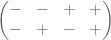
In this case, in the event of obtaining that the balance tips twice to the left: which would be the different stone? The first, which is heaviest, or the fourth, which is lightest? We cannot decide.

One possible solution to this situation involves taking one more measure. Look at the algebraic expression of the following example, to realize why:

$\text{sign} \left[ \begin{pmatrix} 1 & 1 & -1 & -1 \\ 1 & -1 & 1 & -1 \\ 1 & -1 & -1 & 1 \end{pmatrix} \cdot B \right] = \begin{pmatrix} + & + & - & - \\ + & - & + & - \\ + & - & - & + \end{pmatrix}$ or $\begin{pmatrix} - & - & + & + \\ - & + & - & + \\ - & + & + & - \end{pmatrix}$

In this case there is no room for confusion: if the balance tips three times to the same side, then the different stone is the first one (whether heavier or lighter). The other possibilities are also easily solvable: if the balance tips first to one side, then to the other, and then to the first side, then the different stone is the third one.

The reader will not be very surprised at this point to realize that three (non adaptive) measures are also enough to decide which stone is different (be it heavier or lighter) in a set of twelve similar stones. To design the solution, a good weight matrix with twelve columns and three rows need to be constructed. The trick here is to allow measures that balance both plates, which gives us more combinations with which to play. How would the reader design this matrix?

Categories: Combinatorics, Data mining, Linear Algebra, puzzles Tags: balances, compressed sensing, linear algebra, puzzles, weights

Buy my book!

July 20, 2012 Leave a comment

Well, ok, it is not my book technically, but I am one of the authors of one of the chapters. And no, as far as I know, I don’t get a dime of the sales in concept of copyright or anything else.

As the title suggests (Modeling Nanoscale Imaging in Electron Microscopy), this book presents some recent advances that have been made using mathematical methods to resolve problems in electron microscopy. With improvements in hardware-based aberration software significantly expanding the nanoscale imaging capabilities of scanning transmission electron microscopes (STEM), these mathematical models can replace some labor intensive procedures used to operate and maintain STEMs. This book, the first in its field since 1998, covers relevant concepts such as super-resolution techniques (that’s my contribution!), special de-noising methods, application of mathematical/statistical learning theory, and compressed sensing.

We even got a nice review in Physics Today by Les Allen, no less!

Imaging with electrons, in particular scanning transmission electron microscopy (STEM), is now in widespread use in the physical and biological sciences. And its importance will only grow as nanotechnology and nano-Biology continue to flourish. Many applications of electron microscopy are testing the limits of current imaging capabilities and highlight the need for further technological improvements. For example, high throughput in the combinatorial chemical synthesis of catalysts demands automated imaging. The handling of noisy data also calls for new approaches, particularly because low electron doses are used for sensitive samples such as biological and organic specimens.

Modeling Nanoscale Imaging in Electron Microscopy addresses all those issues and more. Edited by Thomas Vogt and Peter Binev at the University of South Carolina (USC) and Wolfgang Dahmen at RWTH Aachen University in Germany, the book came out of a series of workshops organized by the Interdisciplinary Mathematics Institute and the NanoCenter at USC. Those sessions took the unusual but innovative approach of bringing together electron microscopists, engineers, physicists, mathematicians, and even a philosopher to discuss new strategies for image analysis in electron microscopy.

In six chapters, the editors tackle the ambitious challenge of bridging the gap between high-level applied mathematics and experimental electron microscopy. They have met the challenge admirably. I believe that high-resolution electron microscopy is at a point where it will benefit considerably from an influx of new mathematical approaches, daunting as they may seem; in that regard Modeling Nanoscale Imaging in Electron Microscopy is a major step forward. Some sections present a level of mathematical sophistication seldom encountered in the experimentally focused electron-microscopy literature.
The first chapter, by philosopher of science Michael Dickson, looks at the big picture by raising the question of how we perceive nano-structures and suggesting that a Kantian approach would be fruitful. The book then moves into a review of the application of STEM to nanoscale systems, by Nigel Browning, a leading experimentalist in the field, and other well-known experts. Using case studies, the authors show how beam-sensitive samples can be studied with high spatial resolution, provided one controls the beam dose and establishes the experimental parameters that allow for the optimum dose.

The third chapter, written by image-processing experts Sarah Haigh and Angus Kirkland, addresses the reconstruction, from atomic-resolution images, of the wave at the exit surface of a specimen. The exit surface wave is a fundamental quantity containing not only amplitude (image) information but also phase information that is often intimately related to the atomic-level structure of the specimen. The next two chapters, by Binev and other experts, are based on work carried out using the experimental and computational resources available at USC. Examples in chapter four address the mathematical foundations of compressed sensing as applied to electron microscopy, and in particular high-angle annular dark-field STEM. That emerging approach uses randomness to extract the essential content from low-information signals. Chapter five eloquently discusses the efficacy of analyzing several low-dose images with specially adapted digital-image-processing techniques that allow one to keep the cumulative electron dose low and still achieve acceptable resolution.

The book concludes with a wide-ranging discussion by mathematicians Amit Singer and Yoel Shkolnisky on the reconstruction of a three-dimensional object via projected data taken at random and initially unknown object orientations. The discussion is an extension of the authors’ globally consistent angular reconstitution approach for recovering the structure of a macromolecule using cryo-electron microscopy. That work is also applicable to the new generation of x-ray free-electron lasers, which have similar prospective applications, and illustrates nicely the importance of applied mathematics in the physical sciences.

Modeling Nanoscale Imaging in Electron Microscopy will be an important resource for graduate students and researchers in the area of high-resolution electron microscopy.

(Les J. Allen, Physics Today, Vol. 65 (5), May, 2012)


Table of contents	Preface	Sample chapter

Trigonometry

June 22, 2012 Leave a comment

I have just realized that I haven’t posted a good puzzle here in a long time, so here it goes one on Trigonometry, that the average student of Calculus should be able to tackle: you can use anything you think it could help: derivatives, symmetry, periodicity, integration, summation, go to several variables, differential equations, etc

Prove that, for all real values $x \in \mathbb{R},$ it is

$\sin x = x \cos\big(\tfrac{x}{2}\big) \cos\big(\tfrac{x}{4}\big) \cos\big(\tfrac{x}{6}\big) \cos\big(\tfrac{x}{8}\big) \dotsb \cos\big( \tfrac{x}{2n}\big) \dotsb$

or, in a more compact notation,

$\sin x = x \displaystyle{\prod_{n=1}^\infty \cos \big( \tfrac{x}{2n} \big)}$

Categories: Analysis, Geometry, puzzles, Teaching Tags: calculus, cosine, derivatives, infinite sums, integrals, periodicity, product, sine, symmetry, trigonometry

Naïve Bayes

June 21, 2012 Leave a comment

There is nothing naïve about Naïve Bayes—a very basic, but extremely efficient data mining method to take decisions when a vast amount of data is available. The name comes from the fact that this is the simplest application to this problem, upon (the naïve) assumption of independence of the events. It is based on Bayes’ rule of conditional probability: If you have a hypothesis $H$ and evidence $E$ that bears on that hypothesis, then

$\mathrm{Pr} \big( H \lvert E \big) = \displaystyle{ \frac{\mathrm{Pr} \big( E \lvert H\big) \mathrm{Pr}(H)}{\mathrm{Pr}(E)} }$

where as usual, $\mathrm{Pr}(A)$ denotes the probability of the event $A,$ and $\mathrm{Pr}\big( A \lvert B \big)$ denotes the probability of the event $A$ conditional to another event $B.$

I would like to show an example of this technique, of course, with yet another decision-making algorithm oriented to guess my reaction to a movie I have not seen before. From the data obtained in a previous post, I create a simpler table with only those movies that have been scored more than 28 times (by a pool of 87 of the most popular critics featured in www.metacritics.com) [I posted the script to create that table at the end of the post]

Let’s test it:

>>> table=prepTable(scoredMovies,28)
>>> len(table)
49

>>> [entry[0] for entry in table]
[‘rabbit-hole’, ‘carnage-2011’, ‘star-wars-episode-iii—revenge-of-the-sith’,

 ‘shame’, ‘brokeback-mountain’, ‘drive’, ‘sideways’, ‘salt’,

 ‘million-dollar-baby’, ‘a-separation’, ‘dark-shadows’,

 ‘the-lord-of-the-rings-the-return-of-the-king’, ‘true-grit’, ‘inception’,

 ‘hereafter’, ‘master-and-commander-the-far-side-of-the-world’, ‘batman-begins’,

 ‘harry-potter-and-the-deathly-hallows-part-2’, ‘the-artist’, ‘the-fighter’,

 ‘larry-crowne’, ‘the-hunger-games’, ‘the-descendants’, ‘midnight-in-paris’,

 ‘moneyball’, ‘8-mile’, ‘the-departed’, ‘war-horse’,

 ‘the-lord-of-the-rings-the-fellowship-of-the-ring’, ‘j-edgar’,

 ‘the-kings-speech’, ‘super-8’, ‘robin-hood’, ‘american-splendor’, ‘hugo’,

 ‘eternal-sunshine-of-the-spotless-mind’, ‘the-lovely-bones’, ‘the-tree-of-life’,

 ‘the-pianist’, ‘the-ides-of-march’, ‘the-quiet-american’, ‘alexander’,

 ‘lost-in-translation’, ‘seabiscuit’, ‘catch-me-if-you-can’, ‘the-avengers-2012’,

 ‘the-social-network’, ‘closer’, ‘the-girl-with-the-dragon-tattoo-2011’]

>>> table[0]
[‘rabbit-hole’, ”, ‘B+’, ‘B’, ”, ‘C’, ‘C+’, ”, ‘F’, ‘B+’, ‘F’, ‘C’, ‘F’, ‘D’,

 ”, ”, ‘A’, ”, ”, ”, ”, ‘B+’, ‘C+’, ”, ”, ”, ”, ”, ”, ‘C+’, ”, ”,

 ”, ”, ”, ”, ‘A’, ”, ”, ”, ”, ”, ‘A’, ”, ”, ‘B+’, ‘B+’, ‘B’, ”, ”,

 ”, ‘D’, ‘B+’, ”, ”, ‘C+’, ”, ”, ”, ”, ”, ”, ‘B+’, ”, ”, ”, ”, ”,

 ”, ‘A’, ”, ”, ”, ”, ”, ”, ”, ‘D’, ”, ”,’C+’, ‘A’, ”, ”, ”, ‘C+’, ”]

Math still not the answer

May 16, 2012 1 comment

I wrote a quick (but not very elegant) python script to retrieve locally enough data from www.metacritic.com for pattern recognition purposes. The main goal is to help me decide how much I will enjoy a movie, before watching it. I included the script at the end of the post, in case you want to try it yourself (and maybe improve it too!). It takes a while to complete, although it is quite entertaining to see its progress on screen. At the end, it provides with two lists of the same length: critics—a list of str containing the names of the critics; and scoredMovies—a list of dict containing, at index k, the evaluation of all the movies scored by the critic at index k in the previous list.

For example:

>>> critics[43]
‘James White’

>>> scoredMovies[43]
{‘hall-pass’: 60,         ‘the-karate-kid’: 60,  ‘the-losers’: 60,

‘the-avengers-2012’: 80,  ‘the-other-guys’: 60,  ‘shrek-forever-after’: 80,

‘the-lincoln-lawyer’: 80, ‘the-company-men’: 60, ‘jonah-hex’: 40,

‘arthur’: 60,             ‘vampires-suck’: 20,   ‘american-reunion’: 40,

‘footloose’: 60,          ‘real-steel’: 60}

The number of scored films by critic varies: there are individuals that gave their opinion on a few dozen movies, and others that took the trouble to evaluate up to four thousand flicks! Note also that the names of the movies correspond with their web pages in www.metacritic.com. For example, to see what critics have to say about the “Karate Kid” and other relevant information online, point your browser to www.metacritic.com/movie/the-karate-kid. It also comes in very handy if there are several versions of a single title: Which “Karate Kid” does this score refer to, the one in the eighties, or Jackie Chan’s?

Feel free to download a copy of the resulting data [here] (note it is a large file: 1.6MB).

But the fact that we have that data stored locally allows us to gather that information with simple python commands, and perform many complex operations on it.

Sometimes Math is not the answer

April 29, 2012 10 comments

I would love to stand corrected in this case, though. Let me explain first the reason behind this claim—It will take a minute, so bear with me:

Say there is a new movie released, and you would like to know how good it is, or whether you and your partner will enjoy watching it together. There are plenty of online resources out there that will give you enough information to make an educated opinion but, let’s face it, you will not have the complete picture unless you actually go see the movie (sorry for the pun).

For example, I fell for “The Blair Witch Project:” their amazing advertising campaign promised me thrill and originality. On top of that, the averaged evaluation of many movie critics that had access to previews claimed that this was a flick not to be missed… Heck, I even bought the DVD for my sister before even watching it!—She and I have a similar taste with respect to movies. The disappointment was, obviously, epic. Before that, and many a time afterwards, I have tripped over the same stone. If nothing else, I learned not to trust commercials and sneak previews any more (“Release the Kraken!,” anyone?)

The only remaining resource should then be the advice of the knowledgeable movie critics—provided you trust on their integrity, that is. Then it hit me: My taste in movies, so similar to my sister’s, could be completely different to that of the “average critic”. Being that the case, why would I trust what a bunch of experts have to say? The mathematician in me took over, and started planning a potential algorithm:

Categories: Approximation Theory, Data mining, Movies, Scientific Computing, Statistics

What if?

April 11, 2012 Leave a comment

Sara, Spencer and Cam (left to right) discussing their projects in office hour

“What if?” is a truly powerful question. It is the question that separates the child from the adult; the student from the professional. Average students will go through the motions of a course and ask themselves many times: “What is the point of all this?” On the other hand, the notable students on their way to excellence will ask themselves: “How can I profit from this?” It is these inquiring minds who make it at the end: they are a pleasure to work with, they have the drive and the passion to get the job done, enjoy the process, and they are more likely to give their future employers more of their time in pursue of solutions—not because there is monetary or status gain alone, but because their commitment is only matched with their skill and curiosity.

It is a thrill to witness your own students pose that “What if?” question to themselves, and take steps to accomplish that little dream with the knowledge obtained in class. This semester, I had been blessed with a group of extremely talented people in all my different teaching assignments—especially those in my course on elementary differential equations.

Edge detection: The Convolution Approach

November 20, 2011 Leave a comment

Today I would like to show a very basic technique of detection based on simple convolution of an image with small kernels (masks). The purpose of these kernels is to enhance certain properties of the image at each pixel. What properties? Those that define what means to be an edge, in a differential calculus way—exactly as it was defined in the description of the Canny edge detector. The big idea is to assign to each pixel a numerical value that expresses its strength as an edge: positive if we suspect that such structure is present at that location, negative if not, and zero if the image is locally flat around that point. Masks can be designed so that they mimic the effect of differential operators, but these can be terribly complicated and give rise to large matrices.

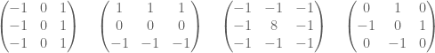
The first approaches were performed with simple $3 \times 3$ kernels. For example, Faler came up with the following four simple masks that emulate differentiation:

$\begin{pmatrix} -1 & 0 & 1\\ -1 & 0 & 1\\ -1 & 0 & 1 \end{pmatrix}\quad \begin{pmatrix} 1 & 1 & 1\\ 0 & 0 & 0 \\ -1 & -1 & -1 \end{pmatrix}\quad \begin{pmatrix} -1 & -1 & -1 \\ -1 & 8 & -1 \\ -1 & -1 & -1 \end{pmatrix}\quad \begin{pmatrix} 0 & 1 & 0 \\ -1 & 0 & 1 \\ 0 & -1 & 0 \end{pmatrix}$

Note that, adding all the values of each matrix, one obtains zero. This is consistent with the third property required for our kernels: in the event of a locally flat area around a given pixel, convolution with any of these will offer a value of zero.

OpArt

September 26, 2011 6 comments

OpArt is, by definition, a style of visual art based upon optical illusions. Let it be a painting, a photograph or any other mean, the objective of this style is to play with the interaction of what you see, and what it really is. A classical OpArt piece involves confusion by giving impression of movement, impossible solids, hidden images, conflicting patterns, warping, etc. And of course, Mathematics is a perfect vehicle to study—and even perform—this form of art.

In this post I would like to show an example of how to use trivial mathematics to implement a well-known example (shown above) in $\LaTeX$ with the tikz package, and leave as homework another more interesting example.

Observe first the image above: the optical effect arises when conflicting concentric squares change the direction of their patterns. You may think that the color is the culprit of this effect but, as you will see below, it is only the relationship between the pure black-and-white patterns what produces the impression of movement.

Categories: Imaging, Scientific Computing, TeX/LaTeX Tags: image, LaTeX, opart, tex, tikz

So you want to be an Applied Mathematician

September 16, 2011 10 comments

The way of the Applied Mathematician is one full of challenging and interesting problems. We thrive by association with the Pure Mathematician, and at the same time with the no-nonsense, hands-in, hard-core Engineer. But not everything is happy in Applied Mathematician land: every now and then, we receive the disregard of other professionals that mistake either our background, or our efficiency at attacking real-life problems.

I heard from a colleague (an Algebrist) complains that Applied Mathematicians did nothing but code solutions of partial differential equations in Fortran—his skewed view came up after a naïve observation of a few graduate students working on a project. The truth could not be further from this claim: we do indeed occasionally solve PDEs in Fortran—I give you that—and we are not ashamed to admit it. But before that job has to be addressed, we have gone through a great deal of thinking on how to better code this simple problem. And you would not believe the huge amount of deep Mathematics that are involved in this journey: everything from high-level Linear Algebra, Calculus of Variations, Harmonic Analysis, Differential Geometry, Microlocal Analysis, Functional Analysis, Dynamical Systems, the Theory of Distributions, etc. Not only are we familiar with the basic background on all those fields, but also we are supposed to be able to perform serious research on any of them at a given time.

My soon-to-be-converted Algebrist friend challenged me—not without a hint of smugness in his voice—to illustrate what was my last project at that time. This was one revolving around the idea of frames (think of it as redundant bases if you please), and needed proving a couple of inequalities involving sequences of functions in $L_p$ —spaces, which we attacked using a beautiful technique: Bellman functions. About ninety minutes later he conceded defeat in front of the board where the math was displayed. He promptly admitted that this was no Fortran code, and showed a newfound respect and reverence for the trade.

It doesn’t hurt either that the kind of problems that we attack are more likely to attract funding. And collaboration. And to be noticed in the press.

Alright, so some of you are sold already. What is the next step? I am assuming that at his point you own your Calculus, Analysis, Probability and Statistics, Linear Programming, Topology, Geometry, Physics and you are able to solve most known ODEs. From here, as with any other field, my recommendation is to slowly build a Batman belt: acquire and devour a sequence of books and scientific articles, until you are very familiar with their contents. When facing a new problem, you should be able to recall from your Batman belt what technique could work best, in which book(s) you could get some references, and how it has been used in the past for related problems.

Following these lines, I have included below an interesting collection with the absolutely essential books that, in my opinion, every Applied Mathematician should start studying:

Smallest Groups with Two Eyes

September 3, 2011 Leave a comment

Today’s riddle is for the Go player. Your task is to find all the smallest groups with two eyes and place them all together (with the corresponding enclosing enemy stones) in a single $19 \times 19$ board. Let me give you some tips first:

Smallest groups in the corner: In the corner, six stones are the minimum needed to complete any group with two eyes. There are only four possibilities, and I took the liberty of placing them on the board for you:
Smallest groups on the side: Consider any of the smallest groups with two eyes on a side of the board. How many stones do they have? [Hint: they all have the same number of stones] How many different groups are there?
Smallest groups in the interior: Consider finally any of the smallest groups with two eyes in the interior of the board. How many stones do they have? [again, they all have the same number of stones]. How many different groups are there?

Since it is actually possible to place all those groups in the same board, this will help you figure out how many of each kind there are. Also, once finished, assume the board was obtained after a proper finished game (with no captures): What is the score?

Categories: Books, Combinatorics, puzzles, TeX/LaTeX Tags: go, LaTeX

The ultimate metapuzzle

August 23, 2011 2 comments

If you have been following this blog for a while, you already know of my fascination with metapuzzles. I have recently found one of the most beautiful examples of these riddles in this August’s edition of Ponder This, and following the advice of Travis, I will leave it completely open for the readers to give it a go. Enjoy!

A mathematician wanted to teach his children the value of cooperation, so he told them the following:

“I chose a secret triangle for which the lengths of its sides are all integers.

To you my dear son Charlie, I am giving the triangle’s perimeter. And to you, my beloved daughter Ariella, I am giving its area.

Since you are both such talented mathematicians, I’m sure that together you can find the lengths of the triangle’s sides.”

Instead of working together, Charlie and Ariella had the following conversation after their father gave each of them the information he promised.

Charlie: “Alas, I cannot deduce the lengths of the sides from my knowledge of the perimeter.”

Ariella: “I do not know the perimeter, but I cannot deduce the lengths of the sides from just knowing the area. Maybe our father is right and we should cooperate after all.”

Charlie: “Oh no, no need. Now I know the lengths of the sides.”

Ariella: “Well, now I know them as well.”

Find the lengths of the triangle’s sides.

Categories: Analysis, Combinatorics, Geometry, puzzles

Where are the powers of two?

June 29, 2011 2 comments

The following construction gives an interesting pairing map between the positive integers and the lattice of integer-valued points in the plane:

Place $\boldsymbol{z}=1$ at the origin.
For each level $n \in \mathbb{N},$ populate the $4n$ points of the plane on the square with vertices $\big\{ (\pm n, 0), (0, \pm n) \big\},$ starting from $z=2(n^2-n+1)$ at the position $(n,0),$ and going counter-clockwise.

After pairing enough positive integers on the lattice, pay attention to the powers of two: they all seem to be located on the same two horizontal lines: $y=0$ and $y=2.$

Is this statement true?

Categories: Analysis, Combinatorics, Geometry, Linear Algebra, puzzles, TeX/LaTeX Tags: pairing functions, puzzles

Geolocation

June 15, 2011 Leave a comment

Recall the First Spherical Law of Cosines:

Given a unit sphere, a spherical triangle on the surface of the sphere is defined by the great circles connecting three points $u$ , $v$ , and $w$ on the sphere. If the lengths of these three sides are $a$ (from $u$ to $v),$ $b$ (from $u$ to $w),$ and $c$ (from $v$ to $w),$ and the angle of the corner opposite $c$ is $C,$ then

$\cos c = \cos a \cos b + \sin a \sin b \cos C$

In any decent device and for most computer languages, this formula should give well-conditioned results down to distances as small as around three feet, and thus can be used to compute an accurate geodetic distance between two given points in the surface of the Earth (well, ok, assuming the Earth is a perfect sphere). The geodetic form of the law of cosines is rearranged from the canonical one so that the latitude can be used directly, rather than the colatitude, and reads as follows: Given points $p_1$ and $p_2$ with positions $(lat_1, long_1)$ and $(lat_2, long_2)$ respectively, the distance $d$ between the two points is given by the following formula.

$\cos\displaystyle{\frac{d}{R_\oplus}}=\sin(lat_1)\sin(lat_2) + \cos(lat_1)\cos(lat_2)\cos(long_2-long_1),$

where $R_\oplus=3,959$ is the radius of the Earth in miles (well, ok, the average radius of the Earth…)

A nice application of this formula can be used for geolocation purposes, and I recently had the pleasure to assist a software company (thumb-mobile.com) to write such functionality for one of their clients.

Go to www.lizardsthicket.com in your mobile device, and click on “Find a Location.” This fires up the location services of your browser. When you accept, your latitude and longitude are tracked. After a fast, reliable and resource-efficient algorithm, the page offers the location of the restaurant from the Lizard’s chain that is closest to you. Simple, right?

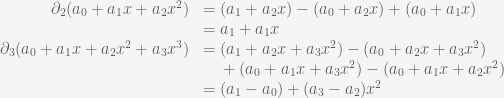
Categories: Geometry, Imaging, Linear Algebra, Scientific Computing Tags: colatitude, geodetic distance, geolocation, latitude, longitude, Sperical Law of Cosines, trigonometry

Boundary operators

May 12, 2011 8 comments

Consider the vector space of polynomials with coefficients on a field $\mathbb{F},$ $\mathbb{F}[X]$ , with the obvious sum of functions and scalar multiplication. For each $n \in \mathbb{N}$ , consider the subspaces $\Pi_n$ spanned by polynomials of order $n$ ,

$\Pi_n = \{ a_0 + a_1 x + \dotsb + a_n x^n : (a_0, a_1, \dotsc, a_n) \in \mathbb{F}^{n+1} \}.$

These subspaces have dimension $n+1.$ Consider now for each $n \in \mathbb{N}$ the maps $\partial_n \colon \Pi_n \to \Pi_{n-1}$ defined in the following way:

$\partial_n \big( a_0 + a_1 x + \dotsb + a_n x^n \big) = \displaystyle{\sum_{k=0}^{n} (-1)^k \sum_{j\neq k} a_j x^{\varphi(j,k)},}$

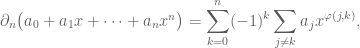
where $\varphi(j,k) = j$ if $j < k,$ and $\varphi(j,k) = j-1$ otherwise.

Schematically, this can be written as follows

$\begin{pmatrix} a_0 \\ a_1 \\ \vdots \\ a_n \end{pmatrix} \xrightarrow{\partial_n} \begin{pmatrix} a_1 \\ a_2 \\ \vdots \\ a_n \end{pmatrix} - \begin{pmatrix} a_0 \\ a_2 \\ \vdots \\ a_n \end{pmatrix} + \dotsb + (-1)^k \begin{pmatrix} \vdots \\ a_{k-1} \\ a_{k+1} \\ \vdots \end{pmatrix} + \dotsb + (-1)^n \begin{pmatrix} a_0 \\ a_1 \\ \vdots \\ a_{n-1} \end{pmatrix},$

and it is not hard to prove that these maps are homeomorphisms of vector spaces over $\mathbb{F}.$

Notice this interesting relationship between $\partial_3$ and $\partial_2:$

$\begin{array}{rl} \partial_2(a_0 + a_1 x + a_2 x^2) &= (a_1 + a_2 x) - (a_0 + a_2 x) + (a_0 +a_1 x) \\ &= a_1 + a_1 x \\ \partial_3( a_0 + a_1 x + a_2 x^2 + a_3 x^3) &= ( a_1 + a_2 x + a_3 x^2 ) - ( a_0 + a_2 x + a_3 x^2) \\ &\mbox{} \quad + (a_0 + a_1 x + a_3 x^2) - (a_0 +a_1 x +a_2 x^2) \\ &= (a_1-a_0) + (a_3-a_2)x^2 \end{array}$

The kernel of $\partial_2$ and the image of $\partial_3$ are isomorphic!

$\begin{array}{rl} \ker \partial_2 &= \{ a_0 + a_2 x^2 : (a_0,a_2) \in \mathbb{F}^2 \}. \\ \partial_3\big( \Pi_3 \big) &= \{ b_0 + b_2 x^2 : (b_0, b_2) \in \mathbb{F}^2 \}. \end{array}$

The reader will surely have no trouble to show that this property is satisfied at all levels: $\ker \partial_n = \partial_{n+1} \big( \Pi_{n+1} \big).$ As a consequence, $\partial_n \partial_{n+1} = 0$ for all $n \in \mathbb{N}.$

We say that a family of homomorphisms $\{ \partial_n \colon \Pi_n \to \Pi_{n+1} \}$ are boundary operators if $\partial_n \partial_{n+1} = 0$ for all $n \in \mathbb{N}.$ If this is the case, then trivially $\partial_{n+1} \big( \Pi_{n+1} \big) \subseteq \ker \partial_n.$ The example above is a bit stronger, because of the isomorphism of both subspaces.

So this is the question I pose as today’s challenge:

Describe all boundary operators $\big\{ \partial_n\colon \Pi_n \to \Pi_{n-1} \big\} \big( \partial_n\partial_{n+1} = 0 \big)$

Include a precise relationship between kernels and images of consecutive maps.

Categories: Analysis, Linear Algebra, puzzles Tags: boundary operator, homomorphism, image, kernel, polynomial, vector space

The Cantor Pairing Function

May 8, 2011 8 comments

The objective of this post is to construct a pairing function, that presents us with a bijection between the set of natural numbers, and the lattice of points in the plane with non-negative integer coordinates.

$\pi\colon \mathbb{N} \cup \{ 0 \} \to \big( \mathbb{N} \cup \{ 0 \} \big)^2.$

We will accomplish this by creating the corresponding map (and its inverse), that takes each natural number $z$ and drops it at a location in the lattice, as the following diagram suggests:

Categories: Analysis, TeX/LaTeX Tags: aleph, bijection, Cantor Pairing function, cardinality, LaTeX, tex, tikz, triangular number

El País’ weekly challenge

April 10, 2011 Leave a comment

For a while now, the Spanish newspaper “El País” has been posing a weekly mathematical challenge to promote a collection of books, and celebrate a hundred years of their country’s Royal Mathematical Society.

The latest of these challenges—the fourth—is a beautiful problem in combinatorics:

Consider a clock, with its twelve numbers around a circle: $1, 2, \dotsc, 12.$ Color each of the twelve numbers in either blue or red, in such a way that there are exactly six in red, and six in blue. Proof that, independently of the order chosen to color the numbers, there always exists a line that divides the circle in two perfect halves, and on each half there will be exactly three numbers in red, and three numbers in blue.

While there are many different ways to solve this challenge, I would like to propose here one that is solely based upon purely counting techniques.

Categories: Combinatorics, puzzles

Math Genealogy Project

February 14, 2011 3 comments

I traced my mathematical lineage back into the XIV century at The Mathematics Genealogy Project. Imagine my surprise when I discovered that a big branch in the tree of my scientific ancestors is composed not by mathematicians, but by big names in the fields of Physics, Chemistry, Physiology and even Anatomy.

There is some “blue blood” in my family: Garrett Birkhoff, William Burnside (both algebrists). Archibald Hill, who shared the 1922 Nobel Prize in Medicine for his elucidation of the production of mechanical work in muscles. He is regarded, along with Hermann Helmholtz, as one of the founders of Biophysics.

Thomas Huxley (a.k.a. “Darwin’s Bulldog”, biologist and paleontologist) participated in that famous debate in 1860 with the Lord Bishop of Oxford, Samuel Wilberforce. This was a key moment in the wider acceptance of Charles Darwin’s Theory of Evolution.

There are some hard-core scientists in the XVIII century, like Joseph Barth and Georg Beer (the latter is notable for inventing the flap operation for cataracts, known today as Beer’s operation).

My namesake Franciscus Sylvius, another professor in Medicine, discovered the cleft in the brain now known as Sylvius’ fissure (circa 1637). One of his advisors, Jan Baptist van Helmont, is the founder of Pneumatic Chemistry and disciple of Paracelsus, the father of Toxicology (for some reason, the Mathematics Genealogy Project does not list any of these two in my lineage—I wonder why).

There are other big names among the branches of my scientific genealogy tree, but I will postpone this discovery towards the end of the post, for a nice punch-line.

Posters with your genealogy are available for purchase from the pages of the Mathematics Genealogy Project, but they are not very flexible neither in terms of layout nor design in general. A great option is, of course, doing it yourself. With the aid of python, GraphViz and a the sage library networkx, this becomes a straightforward task. Let me show you a naïve way to accomplish it:

Categories: sage Tags: genealogy, graph, math genealogy project, mathematics, netowrkx, posters, python, sage

Basic Statistics in sage

February 13, 2011 Leave a comment

No need to spend big bucks in the purchase of expensive statistical software packages (SPSS or SAS): the R programming language will do it all for you, and of course sage has a neat way to interact with it. Let me prove you its capabilities with an example taken from one of the many textbooks used to teach the practice of basic statistics to researchers of Social Sciences (sorry, no names, unless you want to pay for the publicity!)

Estimating Mean Weight Change for Anorexic Girls

The example comes from an experimental study that compared various treatments for young girls suffering from anorexia, an eating disorder. For each girl, weight was measured before and after a fixed period of treatment. The variable of interest was the change in weight; that is, weight at the end of the study minus weight at the beginning of the study. The change in weight was positive if the girl gained weight, and negative if she lost weight. The treatments were designed to aid weight gain. The weight changes for the 29 girls undergoing the cognitive behavioral treatment were

$\begin{array}{rrrrrr} 1.7&0.7&-0.1&-0.7&-3.5&14.9\\3.5&17.1&-7.6&1.6&11.7&6.1\\1.1&-4.0&20.9&-9.1&2.1&1.4\\-0.3&-3.7&-1.4&-0.8&2.4&12.6\\1.9&3.9&0.1&15.4&-0.7\end{array}$

A Homework on the Web System

February 4, 2011 Leave a comment

In the early 2000’s, frustrated with the behavior of most computer-based homework systems in the market, my advisor—Bradley Lucier—decided to take matters into his own hands, and with the help of a couple of students, developed an amazing tool: It generated a great deal of different problems in Algebra and Trigonometry. A single problem model had enough different variations so that no two students would encounter the same exercise in their sessions. It allowed students to input exact answers, rather than mere calculator approximations. It also allowed you to input your answer in any possible legal way. In case of an error, the system would occasionally indicate you where the mistake was produced.

It was solid, elegant, fast… working in this project was sheer delight. The most amazing part of it all: it only took one graduate student to write the codes for the problems and checking for validity of answer. Only two graduate students worked in the coding of this project, with the assistance of several instructors, and Brad himself. He wrote a fun article explaining how the project came to life, enumerating the details that made it so solid, and showing statistical evidence that students working with this environment benefitted more than with traditional methods of evaluation and grading. You can access that article either [here], or continue reading below.

Categories: sage Tags: Brad Lucier, homework on the web, Purdue University

Apollonian gaskets and circle inversion fractals

January 30, 2011 3 comments

Recall the definition of an iterated function system (IFS), and how on occasion, their attractors are fractal sets. What happens when we allow more general functions instead of mere affine maps?

The key to the design of this amazing fractal is in the notion of limit sets of circle inversions.

Toying with basic fractals

January 28, 2011 3 comments

I will skip all the mathematical theory behind Fractals (dimensions, measures, etc) to focus directly into the description and implementation of some of the most basic examples. In this post, I will cover the ideas behind three classical techniques:

Iterated function systems
Membership tests
Lindenmayer systems

Unusual dice

January 27, 2011 Leave a comment

I heard of this problem from Justin James in his TechRepublic post My First IronRuby Application. He tried this fun problem as a toy example to brush up his skills in ruby:

Roll simultaneously a hundred 100-sided dice, and add the resulting values. The set of possible outcomes is, of course, $\{100, 101, \dotsc, 10000\}.$ Note that there is only one way to obtain the outcome 100—all dice showing a 1. There is also only one way to obtain the outcome 10000—all dice showing 100. For the outcome 101, there are exactly 100 different ways to obtain it: all dice except one show a 1, and one die shows a 2. The follow-up question is:

Write a (fast) script that computes the different ways in which we can obtain each of the possible outcomes.

Categories: Combinatorics, Probability, Scientific Computing Tags: combinatorics, dice, ruby, techrepublic

Wavelets in sage

January 23, 2011 2 comments

There are no native wavelet packages in sage. But there is a great module in python that contains, among other things, forward and inverse discrete wavelet transforms (for one and two dimensions). It comes bundled with seventy-six wavelet filters, and allows support to build your own! The name is PyWavelets, written by Tariq Rashid, and can be retrieved from pypi.python.org/pypi/PyWavelets. In order to install it in sage, take the following steps:

Categories: Analysis, Approximation Theory, Imaging, sage, Scientific Computing Tags: python, pywavelet, pywt, sage, wavelets

Edge detection: The Scale Space Theory

January 21, 2011 Leave a comment

Consider an image as a bounded function $f: \square_2 \to \mathbb{R}$ with no smoothness or structure assumptions a priori. Most relevant information of a given image is contained in the contours of the mapped objects: Think for example of a bright object against a dark background—the area where these two meet presents a curve where the intensity $f(\boldsymbol{x})$ varies strongly. This is what we refer to as an “edge.”

Initially, we may consider the process of detection of an edge by the simple computation of the gradient $\nabla f(\boldsymbol{x}) = \big( \tfrac{\partial f}{\partial x_1}, \tfrac{\partial f}{\partial x_2} \big):$ This gradient should have a large intensity $\lvert \nabla f(\boldsymbol{x}) \rvert$ and a direction $\tfrac{\nabla f(\boldsymbol{x})}{\lvert \nabla f(\boldsymbol{x}) \rvert}$ which indicates the perpendicular to the curve. It therefore looks sound to simply compute the gradient of $f$ and choose the points where these values are large. This conclusion is a bit unrealistic for two reasons:

The points where the gradient is larger than a given threshold are open sets, and thus don’t have the structure of curves.
Large gradient may arise in certain locations of the image due to tiny oscillations or noise, but completely unrelated to the objects being mapped. As a matter of fact, there is no reason to assume the existence or computability of any gradient at all in a given digital image.

Bertrand Paradox

January 21, 2011 Leave a comment

Classically, we define the probability of an event as the ratio of the favorable cases, over the number of all possible cases. Of course, these possible cases need to be all equally likely. This works great for discrete settings, like dice rolls, card games, etc. But when facing non-discrete cases, this definition needs to be revised, as the following example shows:

Consider an equilateral triangle inscribed in a circle. Suppose a chord of the circle is chosen at random. What is the probability that the chord is longer than a side of the triangle?

First example Second example Third example

Categories: Geometry, Probability Tags: Euclidean geometry, integral geometry, paradox, probability

Voronoi mosaics

January 4, 2011 Leave a comment

While looking for ideas to implement voronoi in sage, I stumbled upon a beautiful paper written by a group of japanese computer graphic professionals from the universities of Hokkaido and Tokyo: A Method for Creating Mosaic Images Using Voronoi Diagrams. The first step of their algorithm is simple yet brilliant: Start with any given image, and superimpose an hexagonal tiling of the plane. By a clever approximation scheme, modify the tiling to become a voronoi diagram that adaptively minimizes some approximation error. As a consequence, the resulting voronoi diagram is somehow adapted to the desired contours of the original image.


(Fig. 1)	(Fig. 2)	(Fig. 3)	(Fig. 4)

In a second step, they manually adjust the Voronoi image interactively by moving, adding, or deleting sites. They also take the liberty of adding visual effects by hand: emphasizing the outlines and color variations in each Voronoi region, so they look like actual pieces of stained glass (Fig. 4).

Image Processing with numpy, scipy and matplotlibs in sage

December 15, 2010 10 comments

In this post, I would like to show how to use a few different features of numpy, scipy and matplotlibs to accomplish a few basic image processing tasks: some trivial image manipulation, segmentation, obtaining of structural information, etc. An excellent way to show a good set of these techniques is by working through a complex project. In this case, I have chosen the following:

Given a HAADF-STEM micrograph of a bronze-type Niobium Tungsten oxide $Nb_4W_{13}O_{47}$ (left), find a script that constructs a good approximation to its structural model (right).

Courtesy of ETH Zurich

For pedagogical purposes, I took the following approach to solving this problem:

Segmentation of the atoms by thresholding and morphological operations.
Connected component labeling to extract each single atom for posterior examination.
Computation of the centers of mass of each label identified as an atom. This presents us with a lattice of points in the plane that shows a first insight in the structural model of the oxide.
Computation of Delaunay triangulation and Voronoi diagram of the previous lattice of points. The combination of information from these two graphs will lead us to a decent (approximation to the actual) structural model of our sample.

Let us proceed in this direction:

Super-Resolution Micrograph Reconstruction by Nonlocal-Means Applied to HAADF-STEM

May 31, 2010 Leave a comment

We outline a new systematic approach to extracting high-resolution information from HAADF–STEM images which will be beneficial to the characterization of beam sensitive materials. The idea is to treat several, possibly many low electron dose images with specially adapted digital image processing concepts at a minimum allowable spatial resolution. Our goal is to keep the overall cumulative electron dose as low as possible while still staying close to an acceptable level of physical resolution. We wrote a letter indicating the main conceptual imaging concepts and restoration methods that we believe are suitable for carrying out such a program and, in particular, allow one to correct special acquisition artifacts which result in blurring, aliasing, rastering distortions and noise.

Below you can find a preprint of that document and a pdf presentation about this work that I gave in the SEMS 2010 meeting, in Charleston, SC. Click on either image to download.

Categories: Imaging, Scientific Computing Tags: nonlocal means, scanning transmission electron microscopy, STEM, super-resolution

The Nonlocal-means Algorithm

April 28, 2010 Leave a comment

The nonlocal-means algorithm [Buades, Coll, Morel] was designed to perform noise reduction on digital images, while preserving the main geometrical configurations, as well as finer structures, details and texture. The algorithm is consistent under the condition that one can find many samples of every image detail within the same image.


Barbara	Noise added, `std=30`	Denoised image, `h=93`

The algorithm has the following closed form: Given a finite grid $\Lambda \subset \mathbb{Z}^2$ of the form $\Lambda = \Omega \cap \mathbb{Z}^2$ for some compact set $\Omega \subset \mathbb{R}^2$ , a signal $f \in L_2(\Lambda,\mathbb{R}^+)$ , and a family of windows $\{ \mathcal{R}_k \}_{k \in \Lambda}$ satisfying the conditions

$k \in \mathcal{R}_k$ for all $k \in \Lambda$ .
If $j \in \mathcal{R}_k$ , then $k \in \mathcal{R}_j$ ,

the nonlocal-means operator $\text{NL}_h\colon \ell_2(\Lambda,\mathbb{R}) \to \ell_2(\Lambda,\mathbb{R})$ with filtering parameter $h>0$ , is defined by

$\displaystyle{\text{NL}_h f(k) = \sum_{j \in \Lambda} \omega_h(j,k) f(j)},$

where the weights $\{ \omega_h(j,k) \}_{j,k \in \Lambda}$ are defined by

$\displaystyle{ \omega_h(j,k) = \frac{ \exp \bigg( -\frac{\left\lVert f(\mathcal{R}_j) - f(\mathcal{R}_k) \right\rVert_{2,a}^2}{h^2} \bigg) }{ \sum_{j \in \Lambda} \exp \bigg( - \frac{\left\lVert f(\mathcal{R}_j) - f(\mathcal{R}_k) \right\rVert_{2,a}^2}{h^2} \bigg)}. }$

Here, $f(\mathcal{R})$ denotes a patch of the image $f$ supported on the window $\mathcal{R}$ .

Notice that the similarity check between patches is nothing but a simple Gaussian weighted Euclidean distance, which accounts for difference of grayscales alone. Efros and Leung prove that this distance is a reliable measure for the comparison of texture patches, and at the same time copes very well with additive white noise; in particular, if $f$ and $g$ are respectively the noisy and original images, and $\sigma^2$ is the noise variance, then the most similar patches in the noisy image are also expected to be the most similar in the original:

$\mathbb{E} \left\lVert f(\mathcal{R}_j) - f(\mathcal{R}_k) \right\rVert_{2,a}^2 = \left\lVert g(\mathcal{R}_j) - g(\mathcal{R}_k) \right\rVert_{2,a}^2 + 2\sigma^2 .$

Categories: Imaging, Scientific Computing Tags: denoising, nonlocal means, super-resolution

The hunt for a Bellman Function.

September 26, 2008 1 comment

This is a beautiful and powerful mathematical technique in Harmonic Analysis that allows, among other things, to prove very complicated inequalities in the theory of Singular Integral Operators, without using much of the classical machinery in this field.

The Bellman function was the tool that allowed their creators (Fedor Nazarov and Sergei Treil) to crack the problem of weighted norm inequalities with matrix weights for the case $\boldsymbol{p} \neq \boldsymbol{2}$ and finally solve it completely.

Copies of the original paper can be found at the authors’ pages; e.g. [www.math.brown.edu/~treil/papers/bellman/bell3.ps] (notice the postscript file is huge, as the article has more than 100 pages).

Let me illustrate the use of Bellman functions to solve a simple problem:

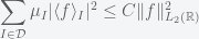
Dyadic- $\boldsymbol{L}_\mathbf{2}(\mathbb{R})$ version of the Carleson Imbedding Theorem

Let $\mathcal{D}$ be the set of all dyadic intervals of the real line. Given a function $f \in L_1^{\text{loc}}(\mathbb{R})$ , consider the averages $\langle f \rangle_I = \lvert I\rvert^{-1} \int_I f$ , on each dyadic interval $I \in \mathcal{D}$ .
Let $\{ \mu_I \geq 0 \colon I \in \mathcal{D} \}$ be a family of non-negative real values satisfying the Carleson measure condition—that is, for any dyadic interval $I \in \mathcal{D}$ , $\sum_{J \subset I, J~\text{dyadic}} \mu_J \leq \lvert I \rvert.$
Then, there is a constant $C>0$ such that for any $f \in L_2(\mathbb{R})$ ,

$\displaystyle{\sum_{ I \in \mathcal{D} } \mu_I \lvert \langle f \rangle_{I} \rvert^2 \leq C \lVert f \rVert_{L_2(\mathbb{R})}^2}$

Categories: Analysis Tags: bellman functions, harmonic analysis, singular integral operators

Presentation: Hilbert Transform Pairs of Wavelets

September 19, 2007 Leave a comment

Now in the stage of the Approximation Theory Seminar, I presented a general overview of the work of Selesnick and others towards the design of pairs of wavelet bases with the “Hilbert Transform Pair property”. Click on the image below to retrieve a pdf file with the slides.

Categories: Analysis Tags: harmonic analysis, signal processing, wavelets

Presentation: The Dual-Tree Complex Wavelet Transform

September 6, 2007 Leave a comment

In the first IMI seminar, I presented an introduction to the survey paper “The Dual-Tree Complex Wavelet Transform“, by Selesnick, Baraniuk and Kingsbury. It was meant to be a (very) basic overview of the usual techniques of signal processing with an emphasis on wavelet coding, an exposition on the shortcomings of real-valued wavelets that affect the work we do at the IMI, and the solutions proposed by the three previous authors. In a subsequent talk, I will give a more mathematical (and more detailed) account on filter design for the dual-tree $\mathbb{C}$ WT. Click on the image below to retrieve a pdf version of the presentation.

Categories: Analysis Tags: harmonic analysis, signal processing, wavelets

Presentation: Curvelets and Approximation Theory

August 5, 2007 1 comment

Find below a set of slides that I used for my talk at the IMA in the Thematic Year on Mathematical Imaging. On them, there is a detailed construction of my generalized curvelets, some results by Donoho and Candès explaining their main properties, and a bunch of applications to Imaging. Click on the slide below to retrieve the pdf file with the presentation.

Categories: Analysis, Approximation Theory, Imaging Tags: approximation theory, curvelets

Poster: Curvelets vs. Wavelets (Mathematical Models of Natural Images)

August 5, 2007 Leave a comment

Together with Professor Bradley J. Lucier, we presented a poster in the Workshop on Natural Images during the thematic year on Mathematical Imaging at the IMA. We experimented with wavelet and curvelet decompositions of 24 high quality photos from a CD that Kodak® distributed in the late 90s. All the experiment details and results can be read in the file Curvelets/talk.pdf.

The computations concerning curvelet coefficients were carried out in Matlab, with the Curvelab 2.0.1 toolbox developed by Candès, Demanet, Donoho and Ying. The computations concerning wavelet coefficients were performed by Professor Lucier’s own codes.

Categories: Analysis, Approximation Theory, Imaging Tags: curvelets, wavelets

Wavelet Coefficients

August 5, 2007 Leave a comment

To aid in my understanding of wavelets, during the first months I started studying this subject I wrote a couple of scripts to both compute wavelet coefficients of a given pgm gray-scale image (the decoding script), and recover an approximation to the original image from a subset of those coefficients (the coding script). I used OCaml, a multi-paradigm language: imperative, functional and object-oriented.

The decoding script uses the easiest wavelets possible: the Haar functions. As it was suggested in the article “Fast wavelet techniques for near-optimal image processing“, by R. DeVore and B.J. Lucier, rather than computing the actual raw wavelet coefficients, one computes instead a related integer value (a code). The coding script interprets those integer values and modifies them appropriately to obtain the actual coefficients. The storage of the integers is performed using Huffman trees, but I used a very simple one, not designed for speed or optimization in any way.

Following a paper by A.Chambolle, R.DeVore, N.Y.Lee and B.Lucier, “Non-linear wavelet image processing: Variational problems, compression and noise removal through wavelet shrinkage“, these scripts were used in two experiments later on: computation of the smoothness of an image, and removal of Gaussian white noise by the wavelet shrinkage method proposed by Donoho and Johnstone in the early 90’s.

Progressive reconstruction of a grey-scale image of size $1024 \times 1024$ with the largest (in absolute value) $2^n$ coefficients, $n = 1,2, \dotsc ,8.$

Categories: Analysis, Approximation Theory, Scientific Computing Tags: wavelets

Modeling the Impact of Ebola and Bushmeat Hunting on Western Lowland Gorillas

August 5, 2007 Leave a comment

In May 2003, together with fellow Mathematician Stephanie Gruver, Statistician Young-Ju Kim, and Forestry Engineer Carol Rizkalla, we worked on this little project to apply ideas from Dynamical Systems to an epidemiology model of the Ebola hemorrhagic fever in the Republic of Congo. The manuscript ebola/root.pdf is a first draft, and contains most of the mathematics behind the study. Carol worked in a less-math-more-biology version: ebola/Ecohealth.pdf “Modeling the Impact of Ebola and Bushmeat Hunting on Western Lowland Gorillas,” and presented it to EcoHealth, where it has been published (June 2007). She also prepared a poster for the Sigma-Xi competition: Click on the image below to retrieve a PowerPoint version of it.

Categories: Scientific Computing Tags: dynamical systems, ebola, epidemiology

Triangulations

August 5, 2007 Leave a comment

As part of a project developed by Professor Bradley J. Lucier, to code a PDE solver written in scheme, I worked in some algorithms to perform “good triangulations” of polygons with holes (“good triangulations” meaning here, those where all the triangles have their three angles as close to 60º as possible). I obtained the necessary theoretical background and coding strategies from the following references:

Mark de Berg et al., “Computational Geometry by Example.“
Francis Chin and Cao An Wang, “Finding the Constrained Delaunay Triangulation and Constrained Voronoi Diagram of a simple Polygon in Linear Time.“
Joseph O’Rourke, “Computational Geometry in C.“
Jim Ruppert, “A Delaunay Refinement Algorithm for Quality 2-dimensional Mesh Generation.“

Categories: Geometry, Scientific Computing Tags: computational geometry, triangulation, voronoi diagram

Mechanical Geometry Theorem Proving

August 5, 2007 1 comment

In 1977, Professor Wen-Tsun Wu succeeded in developing a method of mechanical geometry theorem proving. This method has been applied to prove or even discover hundreds of non-trivial difficult theorems in elementary and differential geometries on a computer in an almost trivial manner. Usign Ritt’s differential algebra, Wu established a method for solving algebraic and differential equations by transforming an equation system in the general form to equation systems in triangular form. This is the Ritt-Wu decomposition algorithm, that later on was shown to be equivalent to perform a series of operations on ideals, very easily carried out by means of Gröbner basis manipulation.

I wrote a script in MAPLE to perform evaluations of the validity of some simple theorems in Euclidean Geometry, and wrote a small paper (in Spanish) on one of my findings, that was published in Bol. Asoc. Prof. Puig Adams, in October’99: “Sobre demostración automática de un problema geométrico“.

The example I cover in that short article can be seen below.

Given: Circles $A$ , $B$ that intersect each other in points $C$ and $D$ , and given points $E$ , $F$ in circle $A$ , consider line $a$ through $E$ and $C$ , and line $b$ through $F$ and $D$ . The intersections of line $a$ with circle $A$ are $C$ and $G$ . The intersections of line $b$ with circle $B$ are $D$ and $H$ . Consider the segments $c$ (connecting $E$ with $F$ ) and $d$ (connecting $G$ with $H$ ).

To prove: Segments $c$ and $d$ are parallel.

Categories: Geometry Tags: Euclidean geometry, mechanical theorem proving, Ritt-Wu

Share this:

Share this:

Share this:

Share this:

Talk the talk

Walk the walk

Sing me a song

Share this:

Share this:

Share this:

Share this:

Share this:

Share this:

Share this:

Share this:

Share this:

Share this:

Share this:

Share this:

Share this:

Share this:

Share this:

Share this:

Share this:

Share this:

Share this:

Share this:

Share this:

Share this:

Share this:

Share this:

Share this:

Share this:

Share this:

Share this:

Share this:

Share this:

Share this:

Share this:

Share this:

Estimating Mean Weight Change for Anorexic Girls

Share this:

Share this:

Share this:

Share this:

Share this:

Share this:

Share this:

Share this:

Share this:

Share this:

Share this:

Share this:

Share this:

Share this:

Share this:

Share this:

Share this:

Share this:

Share this:

Share this:

Share this:

We have moved!

Blanco-Silva’s Books

In the news:

Recent Posts

Pages

Categories

Archives

Email Subscription